DADA2 ASVs pipeline, ITS2 

This example data analyses follows vsearch OTUs workflow as implemented in PipeCraft2’s pre-compiled pipelines panel.

Download example data set here (15.1 Mb) and unzip it.

This is ITS2 Illumina MiSeq dataset.

For this example, we are using EUKARYOME database in the taxonomy annotation process Download the General_EUK_ITS file from here and unzip it (note: use 7-Zip software for unzipping files in Windows).

Starting point

This example dataset consists of ITS2 rRNA gene amplicon sequences; targeting fungi:

paired-end Illumina MiSeq data;
demultiplexed set (per-sample fastq files);
primers are not removed;
sequences in this set are 5’-3’ oriented.

when working with your own data …

… then please check that the paired-end data file names contain R1 and R2 strings (not just _1 and _2), so that PipeCraft can correctly identify the paired-end reads.

Example:
sample1_R1.fastq.gz
sample1_R2.fastq.gz

To select DADA2 pipeline, press

SELECT PIPELINE –> DADA" ASVs.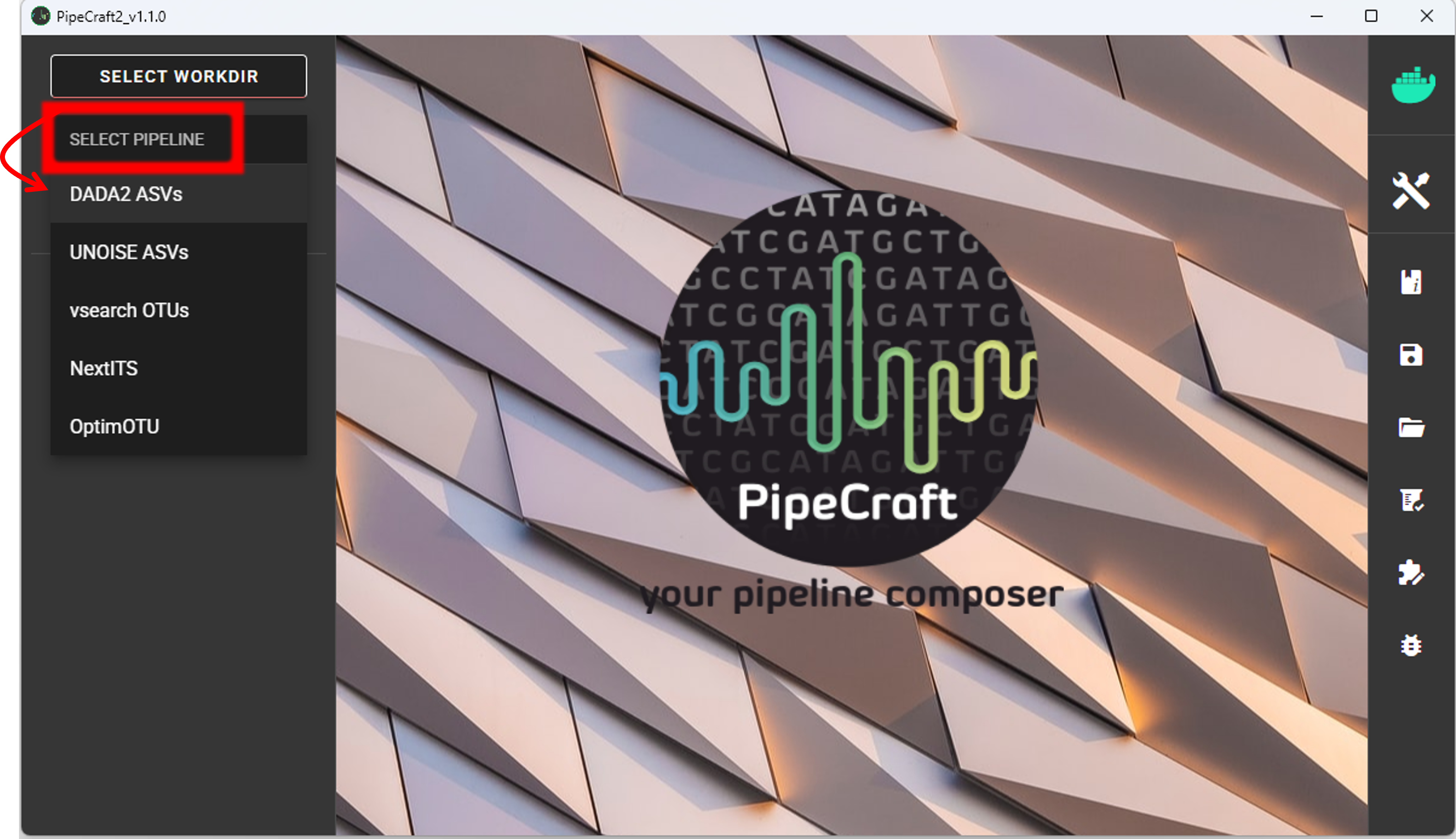

To select input data, press SELECT WORKDIR
and specify
sequence files extension as *.fastq.gz;
sequencing read types as paired-end.

Workflow mode

Because we are working with sequences that are 5’-3’ oriented, we are selecting hte PAIRED-END FORWARD mode of the pipeline.

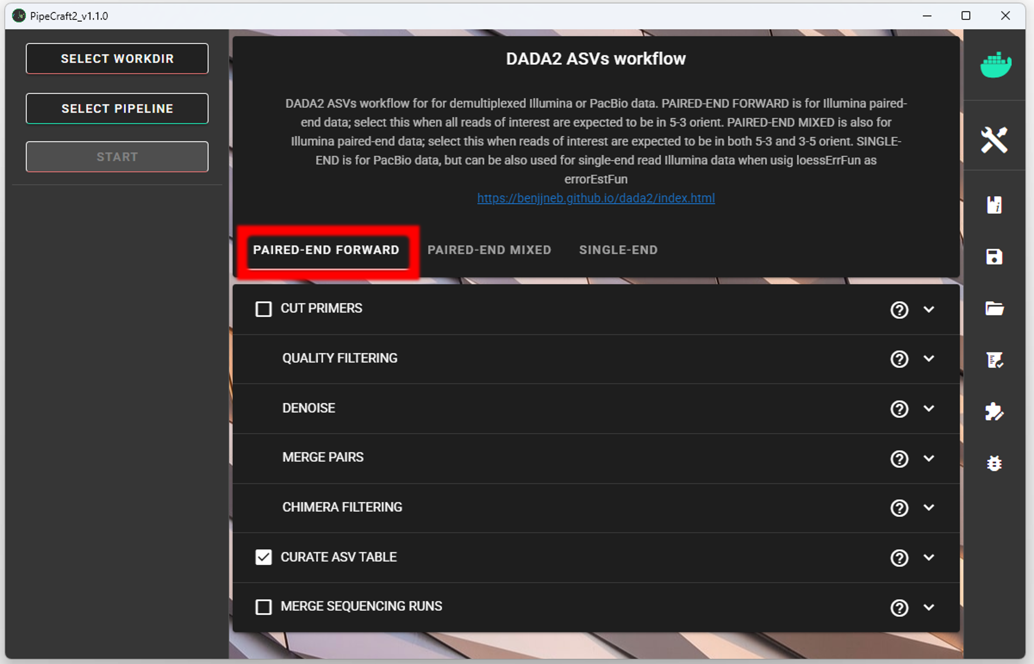
if sequences are in mixed orientation

If some sequences in your library are in 5’-3’ and some as 3’-5’ orientation, then with the ‘PAIRED-END FORWARD’ mode exactly the same ASV may be reported twice, where one ASV is just the reverse complementary of another. To avoid that, select PAIRED-END MIXED mode. Sequences have mixed orientation in libraries where sequenceing adapters have been ligated, rather than attached to amplicons during PCR.

Specifying primers (for CUT PRIMERS) is mandatory for the PAIRED-END MIXED mode. Based on the priemr sequences, the library will be split into two: 1) fwd oriented sequences, and 2) rev oriented sequences. Both batches are processed independently to produce ASVs, after which the rev oriented batch ASVs are reverse complemented and merged with the fwd oriented ASVs. Identical ASVs are merged to form a final data set. This is a reccomended workflow for accurate denoising compared with first reorienting all sequences to 5’-3’, and then performing a standard ‘PAIRED-END FORWARD’ workflow.

Cut primers

Although the sequences in the example dataset are containing primer sequences, we are not clipping those here because we will later use the ITSx step to remove the flanking primer binding regions from ITS reads.

when working with your own data …

… and you need to clip primers, then check the box for CUT PRIMERS and specify the PCR primers. You may specify add up to 13 primer pairs. Check cut primers page.

Quality filtering

Before adjusting quality filtering settings, let’s have a look on the quality profile of our example data set. Below quality profile plot was generated using QualityCheck panel (see here).

…

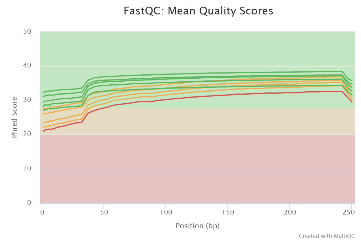
Denoise and merge pairs

This step performs desiosing (as implemented in DADA2), which first forms ASVs per R1 and R2 files. Then during merging/assembling process the paired ASV mates are assembled to output full amplicon length ASV.

Chimera filtering

This step performs chimera filtering according to DADA2 removeBimeraDenovo function. During this step, the ASV table is also generated.

Important

make sure that primers have been removed from your amplicons; otherwise many false-positive chimeras may be filtered out from your dataset.

Here, we filter chimeras using the consensus method.

Output directory	`chimeraFiltered_out.dada2`
*.fasta	chimera filtered ASVs per sample
seq_count_summary.csv	summary of sequence counts per sample
‘chimeras’ dir	ASVs per sample identified as chimeras

Output directory	`ASVs_out.dada2`
ASVs_table.txt	denoised and chimera filtered ASV-by-sample table
ASVs.fasta	corresponding FASTA formated ASV Sequences
ASVs per sample identified as chimeras	rds formatted denoised and chimera filtered ASV table

Curate ASV table

This process first removes putative tag jumps and then collapses the ASVs that are identical up to shifts or length variation, i.e. ASVs that have no internal mismatches; and finally filters out ASVs that are shorter/longer than specified length (in base pairs).

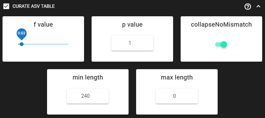
Here, we are enabling this process by checking the box for CURATE ASV TABLE in the DADA2 ASV workflow panel.

The f_value and p_value settings are used to filter out putative tag jumps (using UNCROSS2 algorithm). Generally, we recommend to use p_value of 1 (default), and f_value of 0.03 when using combinational indexing strategy; f_value of 0.05 when using single-indexes, and f_value of 0.01 when using unique dual-indexes.

The expected amplicon length (without primers) in our example dataset in ~253 bp. Assuming that shorter sequences are non-target sequences, we use 240 in the min length setting. This will discard ASVs that are less than 240 bp. Here, max length can be set to 0 (default), meaning no filtering by maximum sequence length.

We are also setting hte collapseNoMismatch to TRUE, to collapse identical ASVs. This is basically equivalent to 100% clustering by ignoring the end gaps.

Output directory `ASVs_out.dada2/curated`
ASVs_collapsed.fasta	tag-jump filtered and collapsed and size filtered ASV Sequences
ASVs_table_collapsed.txt	corresponding ASV-by-sample table (curated)
ASVs_table_TagJumpFilt.txt	only tag-jump filtered ASV-by-sample table
ASVs.fasta	corresponding ASV Sequences with ASVs_table_TagJumpFilt.txt table

If there is nothing to collapse or filter out based on the length

then there are no corresponding files in the ASVs_out.dada2/curated directory, and only ASVs_table_TagJumpFilt.txt and ASVs.fasta files will be generated (even when there is nothing to tag-jump filter - in which case ASVs_table_TagJumpFilt.txt is the same ASVs_table.txt in the ASVs_out.dada2 directory).

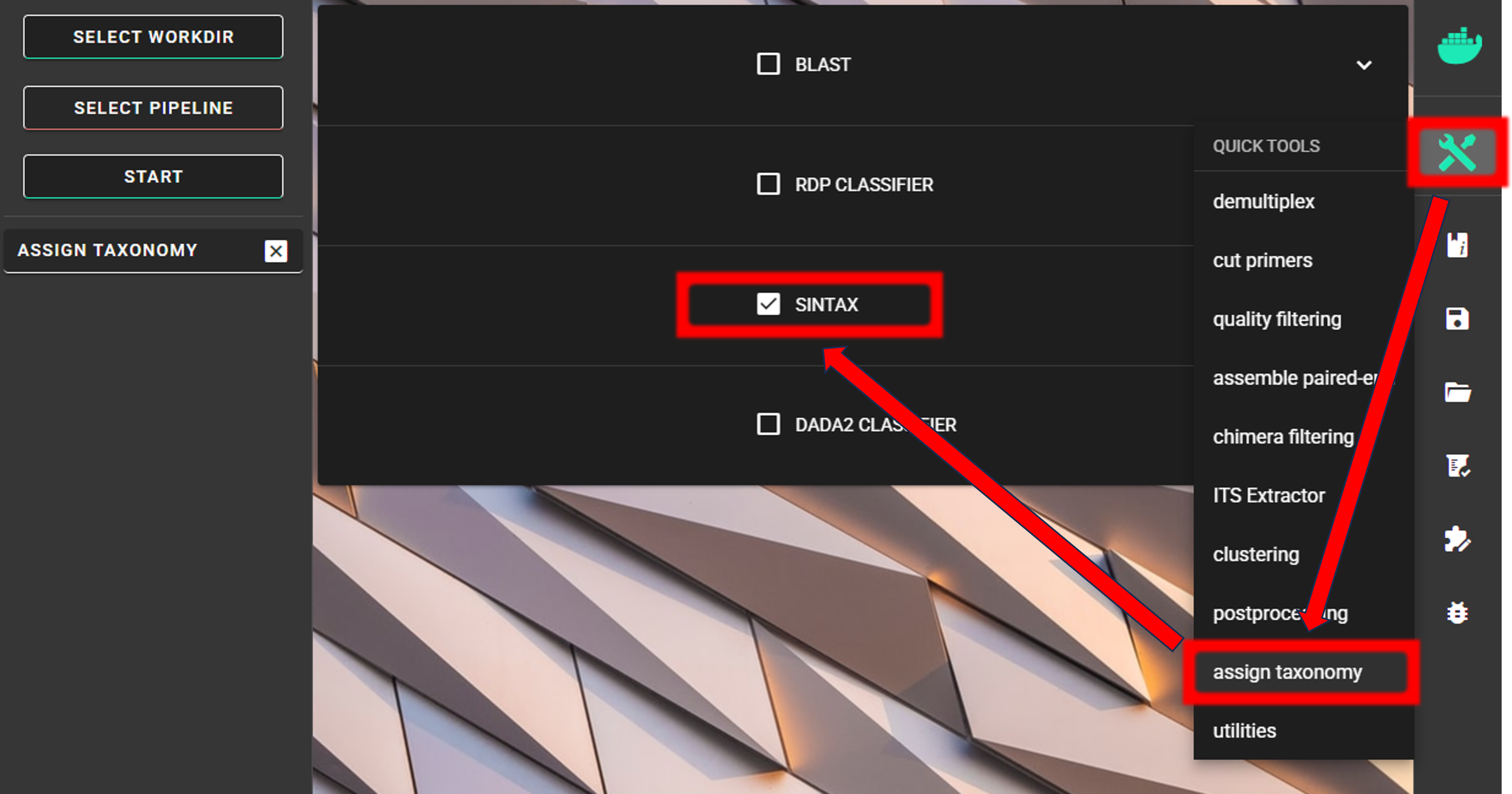
Assign taxonomy

Assign taxonomy is not the part of the full per-defined pipeline, but can be run as a separate step in QuickTools. Here, we are using the SINTAX classifier for that.

Save workflow

Once we have decided about the settings in our workflow, we can save the configuration file by pressing save workflow button on the right-ribbon.

If you forget the save, then no worries, a pipecraft2_last_run_configuration.json file will be generated for you upon starting the workflow. As the file name says, it is the workflow configuration file for your last PipeCraft run in this working directory. If the file name (pipecraft2_last_run_configuration.json) is not changed, then the file is overwritten with the new configuration if running a new job in the same working directory.

This JSON file can be loaded into PipeCraft2 to automatically configure your next runs exactly the same way.

Start the workflow

Press START on the left ribbon to start the analyses.

when running the module for the first time …

… a docker image will be first pulled to start the process.

For example:

When you need to STOP the workflow, press STOP button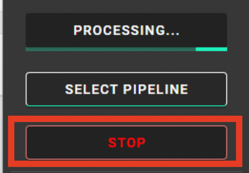

When the workflow has completed …

… a message window will be displayed.