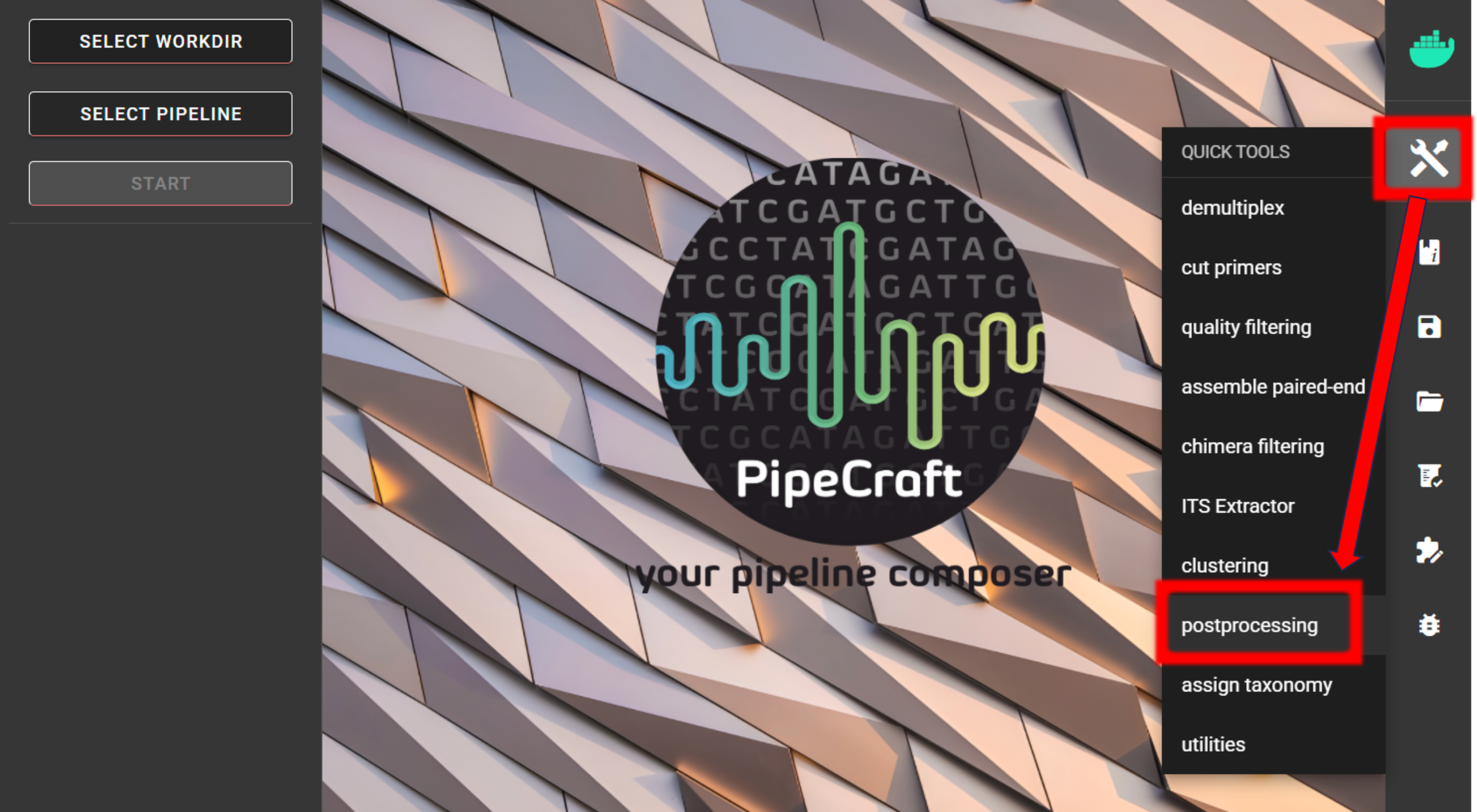
Post-processing tools 

All post-processing tools accessible under QuickTools -> Postprocessing

Filter tag-jumps

Filter out putative tag-jumps with UNCROSS2. This is done via QuickTools -> Postprocessing -> FILTER TAG-JUMPS, but is also automatically performed as a part of the pre-compiled pipelines via CURATE ASV/OTU TABLE panel by specifying f-value and p-value parameters (see here).

Tag-jumps (also called index/tag switching or sample cross-talk) are library-preparation/sequencing artifacts where a small fraction of reads are assigned the wrong sample index. This creates low-level “ghost” occurrences of real sequences in samples where they are not truly present. If not removed, tag-jumps can inflate apparent diversity, introduce false positives (especially in low-biomass samples), which may bias downstream analyses. Tag-jumps filtering aims to remove these low-frequency cross-sample contaminants.

Input data

Input data is tab delimited OTU/ASV table and corresponding fasta file (representative sequences of ASV/OTUs). Note that the input FASTA file is not changed: tag-jumps filtering does not delete ASVs/OTUs globally. Instead, it adjusts the feature table by removing (setting to zero) low-abundance occurrences of a feature in specific samples where they are likely due to tag-jumps. Here, FASTA file is only used to add sequences (back) to the feature table after filtering. This is needed for example when subjecting the resulting feature table to further clustering (see ASV TO OTU).

The input table format; can contain “Sequence” column (but this is ignored):

ASV	Sequence	Sample_1	Sample_2	Sample_3	…
ASV_1	ATGCTGATC…	0	200	320	…
ASV_2	ATGCTGATC…	99	200	222	…
ASV_3	ATGCTGATC…	10	34	3	…

To START

To START, specify working directory under SELECT WORKDIR (outputs will be written here), but the following requests about Sequence files extension and Sequencing read types do not matter here, just click ‘Confirm’.

Settings

Setting	Tooltip
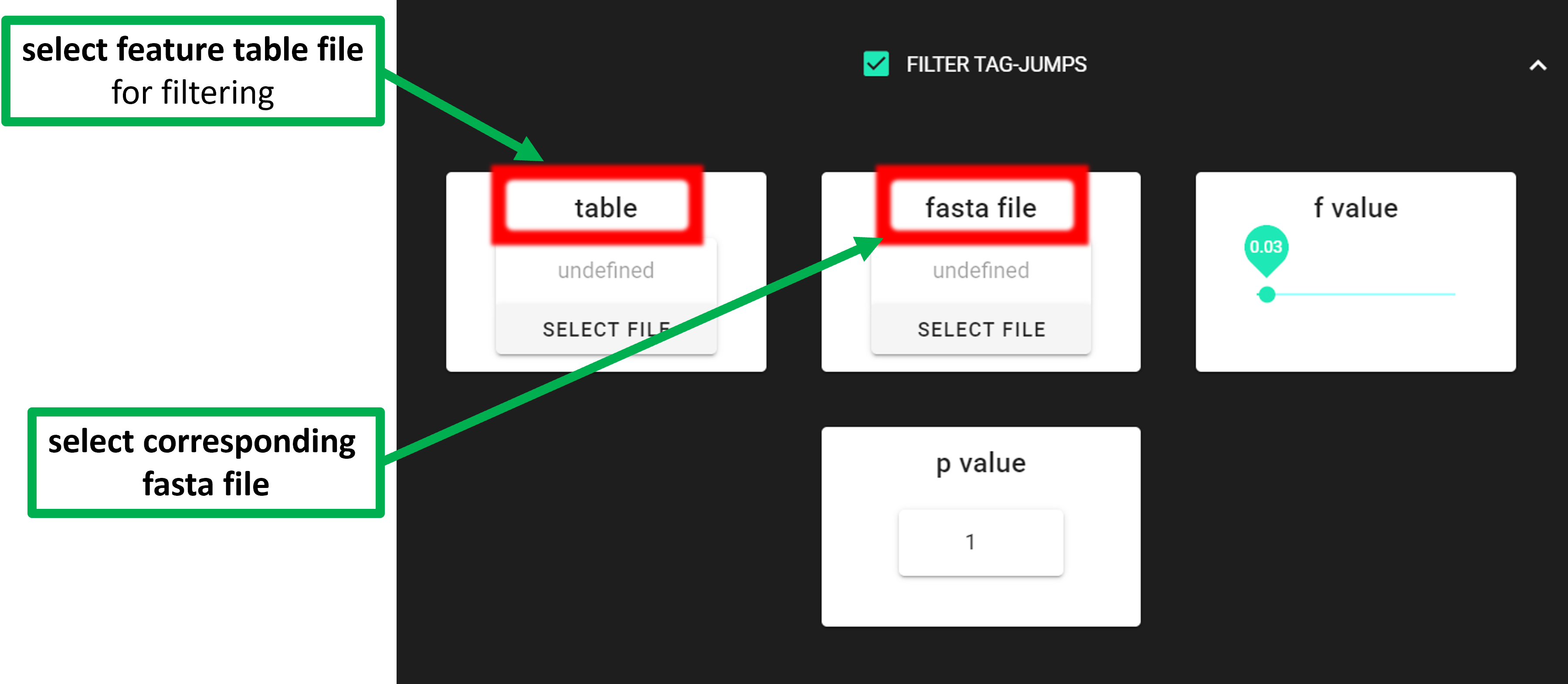
`table`	select tab-delimited OTU/ASV table, where the 1st column is the OTU/ASV IDs and the following columns represent samples; 2nd column may be Sequence column, with the colName ‘Sequence’ [file must be in the SELECT WORKDIR directory]
`fasta file`	select corresponding fasta file for OTU/ASV table [fasta file must be in the SELECT WORKDIR directory]
`f value`	f-parameter of UNCROSS2, which defines the expected tag-jumps rate. Default is 0.03 (equivalent to 3%). A higher value enforces stricter filtering
`p value`	p-parameter, which controls the severity of tag-jump removal. It adjusts the exponent in the UNCROSS formula. Default is 1. Opt for 0.5 or 0.3 to steepen the curve

The f value and p value settings are used to filter out putative tag jumps (using UNCROSS2 algorithm). Generally, we recommend to use p_value of 1 (default), and f_value of 0.03 when using combinational indexing strategy; f_value of 0.05 when using single-indexes, and f_value of 0.01 when using unique dual-indexes.

Outputs

Outputs are in the selected working directory:

Outputs
`*_TagJumpFilt.txt`	output table where tag-jumps have been filtered out
TagJump_plot.pdf	illustration about the presence of tag-jumps based on the selected parameters
TagJump_stats.txt	tag-jump statistics (Total_reads, Number_of_TagJump_Events, TagJump_reads, ReadPercent_removed)

ASV to OTU

Cluster ASVs (or zOTUs) to OTUs.

If the aim is to work on OTU-level, but also benefit from the denoising workflows as implemented in DADA2 or UNOISE pipelines (that produce ASVs), then resulting ASVs can be clustered to OTUs (using vsearch). This is done via QuickTools -> Postprocessing -> ASV TO OTU.

Input data

Input data is ASV sequences in fasta format and corresponding tab delimited ASV table file. 2nd column of the ASV table MUST BE ‘Sequences’ (1st column is ASV IDs; default pipecraft output table). For clustering, the ASV size annotation is obtained from the ASV table.

If the ASV table does not contain ‘Sequence’ column, then add those with QuickTools -> Utilities -> Add sequences to table see here.

It is allowed that the selected fasta file (ASV fasta) contains a subset of ASVs that are present in the provided table file (ASV table). The clustering will be applied to the ASVs in the fasta file. This enables to cluster ASVs if, for example, ITSx is applied after DADA2 ASVs pipeline, and some ASVs are discarded by ITSx (i.e., no ITS region detected).

The input table format; MUST contain “Sequence” column:

ASV	Sequence	Sample_1	Sample_2	Sample_3	…
ASV_1	ATGCTGATC…	0	200	320	…
ASV_2	ATGCTGATC…	99	200	222	…
ASV_3	ATGCTGATC…	10	34	3	…

To START

To START, specify working directory under SELECT WORKDIR (outputs will be written here), but the following requests about Sequence files extension and Sequencing read types do not matter here, just click ‘Confirm’.

Settings

Setting	Tooltip
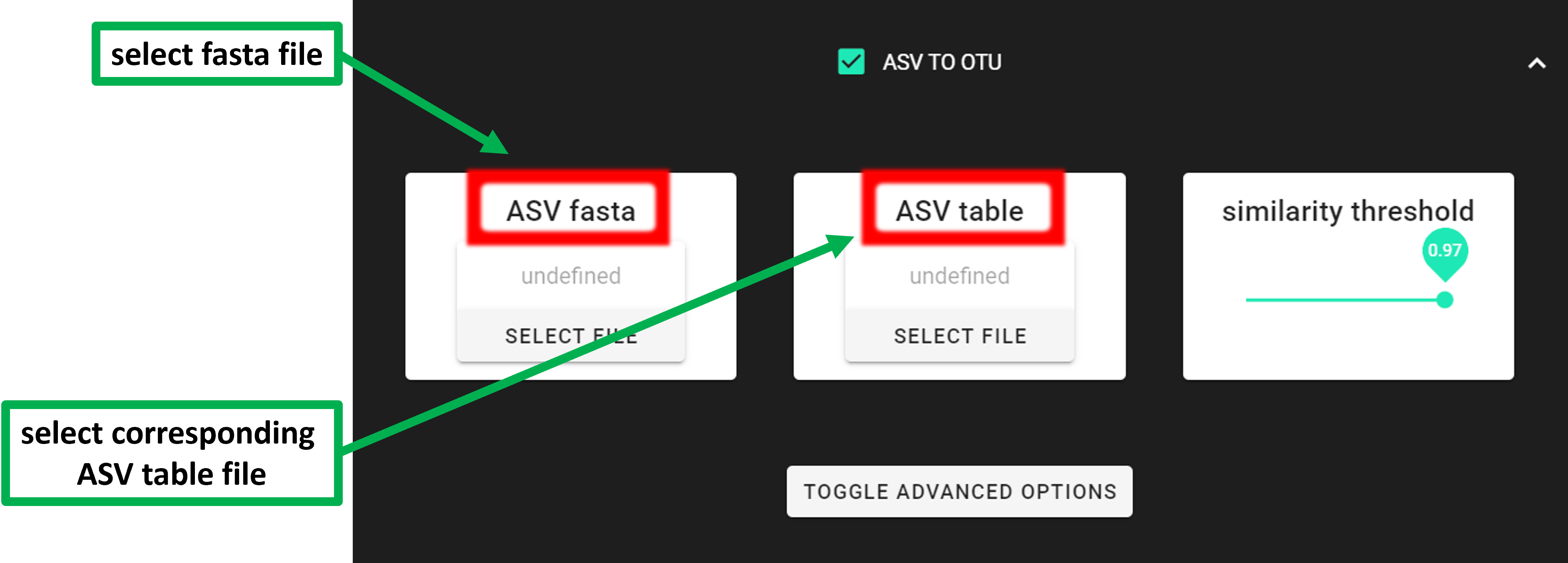
`ASV fasta`	select fasta formatted ASVs sequence file (ASV IDs must match with the ones in the ASVs table) [fasta file must be in the SELECT WORKDIR directory]
`ASV table`	select ASVs_table file [1st col is ASVs ID, 2nd col MUST BE ‘Sequences’ (default PipeCraft’s output)] [file must be in the SELECT WORKDIR directory]
`similarity threshold`	define OTUs based on the sequence similarity threshold; 0.97 = 97% similarity threshold
`OTU type`	“centroid” = output centroid sequences; “consout” = output consensus sequences
`strands`	when comparing sequences with the cluster seed, check both strands (forward and reverse complementary) or the plus strand only
`remove singletons`	remove singleton OTUs (e.g., if TRUE, then OTUs with only one sequence will be discarded)
`similarity type`	pairwise sequence identity definition (–iddef of vsearch)
`sequence sorting`	size = sort the sequences by decreasing abundance; “length” = sort the sequences by decreasing length (–cluster_fast); “no” = do not sort sequences (–cluster_smallmem –usersort)
`centroid type`	“similarity” = assign representative sequence to the closest (most similar) centroid (distance-based greedy clustering); “abundance” = assign representative sequence to the most abundant centroid (abundance-based greedy clustering; –sizeorder), –maxaccepts should be > 1
`maxaccepts`	maximum number of hits to accept before stopping the search (should be > 1 for abundance-based selection of centroids [centroid type])
`mask`	mask regions in sequences using the “dust” method, or do not mask (“none”).

Outputs

Outputs are in ASVs2OTUs_out directory:

Outputs `ASVs2OTUs_out`
OTUs.fasta	FASTA formated representative OTU sequences
OTU_table.txt	OTU distribution table per sample (tab delimited file)
OTUs.uc	uclust-like formatted clustering results for OTUs
ASVs.size.fasta	size annotated input sequences

LULU post-clustering

Perform OTU post-clustering with LULU to merge co-occurring ‘daughter’ OTUs; QuickTools -> Postprocessing -> LULU.

LULU description from the LULU repository: the purpose of LULU is to reduce the number of erroneous OTUs in OTU tables to achieve more realistic biodiversity metrics. By evaluating the co-occurence patterns of OTUs among samples LULU identifies OTUs that consistently satisfy some user selected criteria for being errors of more abundant OTUs and merges these. It has been shown that curation with LULU consistently result in more realistic diversity metrics.

Input data

Input data is tab delimited OTU table (table) and OTU sequences (rep_seqs) in fasta format.

The input table format; can contain “Sequence” column (but this is ignored):

OTU	Sequence	Sample_1	Sample_2	Sample_3	…
OTU_1	ATGCTGATC…	0	200	320	…
OTU_2	ATGCTGATC…	99	200	222	…
OTU_3	ATGCTGATC…	10	34	3	…

To START

To START, specify working directory under SELECT WORKDIR (outputs will be written here), but the following requests about Sequence files extension and Sequencing read types do not matter here, just click ‘Confirm’.

Settings

Setting	Tooltip
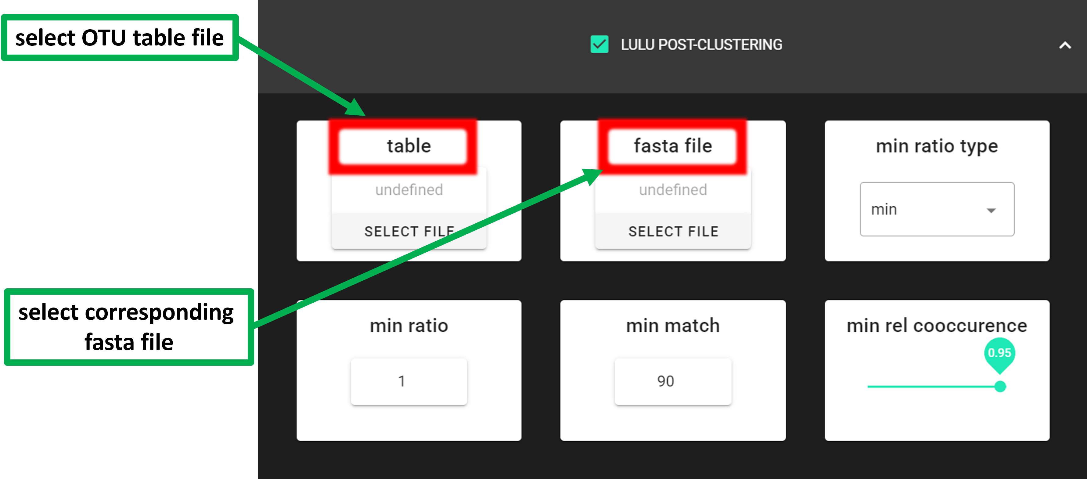
`table`	select OTU/ASV table. If no file is selected, then PipeCraft will look OTU_table.txt or ASV_table.txt in the working directory. EXAMPLE table here
`fasta_file`	select fasta formatted sequence file containing your OTU/ASV reads. EXAMPLE file here
`min_ratio_type`	sets whether a potential error must have lower abundance than the parent in all samples ‘min’ (default), or if an error just needs to have lower abundance on average ‘avg’
`min_ratio`	set the minimim abundance ratio between a potential error and a potential parent to be identified as an error
`min_match`	specify minimum threshold of sequence similarity for considering any OTU as an error of another
`min_rel_cooccurence`	minimum co-occurrence rate. Default = 0.95 (meaning that 1 in 20 samples are allowed to have no parent presence)
`match_list_soft`	use either ‘blastn’ or ‘vsearch’ to generate match list for LULU. Default is ‘vsearch’ (much faster)
`vsearch_similarity_type`	applies only when ‘vsearch’ is used as ‘match_list_soft’. Pairwise sequence identity definition (–iddef)
`perc_identity`	percent identity cutoff for match list. Excluding pairwise comparisons with lower sequence identity percentage than specified threshold
`coverage_perc`	percent query coverage per hit. Excluding pairwise comparisons with lower sequence coverage than specified threshold
`strands`	query strand to search against database. Both = search also reverse complement

Outputs

Outputs are in lulu_out directory:

Outputs `lulu_out`
OTU_table.lulu.txt	curated table in tab delimited txt format
OTUs.lulu.fasta	fasta file for the molecular units (OTUs or ASVs) in the curated table
match_list.lulu	match list file that was used by LULU to merge ‘daughter’ molecular units
discarded_units.lulu	molecular units (OTUs or ASVs) that were merged with other units based on specified thresholds

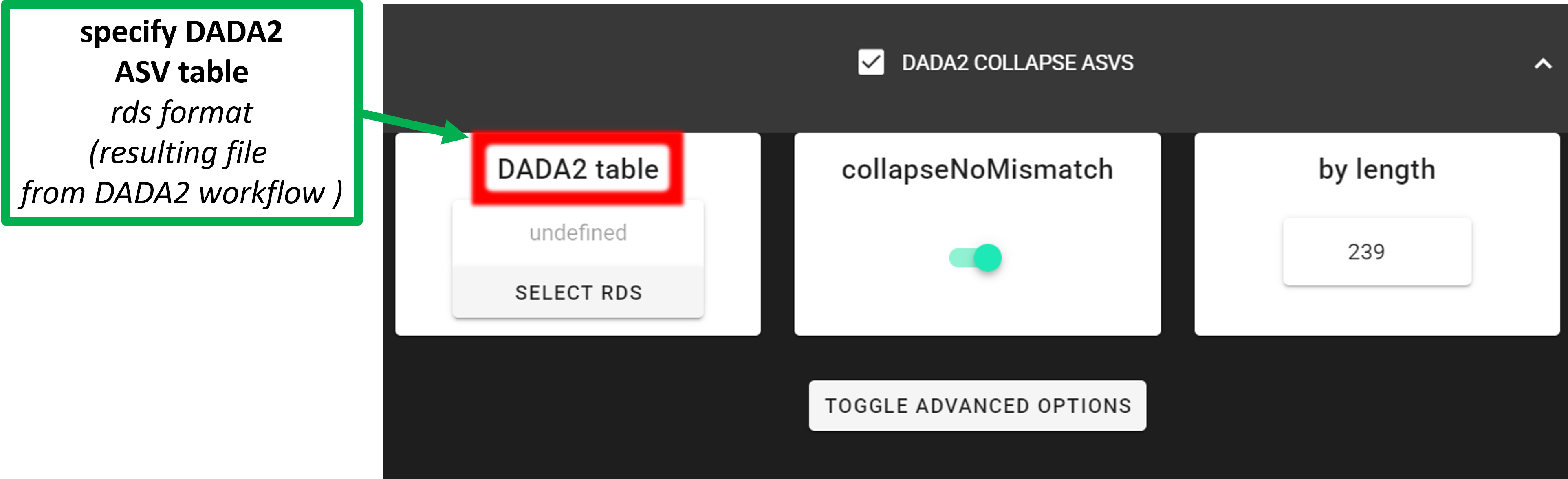
DADA2 collapse ASVs

DADA2 collapseNoMismatch function collapses identical ASVs with no internal mismatches (~greedy 100% clustering with end-gapping ignored). Representative sequence of a collapsed ASV will be the most abundant one.

Input data

Input data is DADA2 compatible RSD table file resulting from DADA2 workflow (in dir ASVs_out.dada2).

This process can be automatically performed also by setting the collapseNoMismatch = TRUE while running the DADA2 pre-compiled pipeline (see here).

To START

To START, specify working directory under SELECT WORKDIR (outputs will be written here), but the following requests about Sequence files extension and Sequencing read types do not matter here, just click ‘Confirm’.

Settings

Setting	Tooltip
`DADA2 table`	select the RDS file (ASV table), output from DADA2 workflow; usually in ASVs_out.dada2/ASVs_table.*.rds
`collapseNoMismatch`	collapses ASVs that are identical up to shifts or length variation, i.e. that have no mismatches or internal indels
`by_length`	discard ASVs from the ASV table that are shorter than specified value (in base pairs). Value 0 means OFF, no filtering by length
`minOverlap`	collapseNoMismatch setting. Default = 20. The minimum overlap of base pairs between ASV sequences required to collapse them together
`vec`	collapseNoMismatch setting. Default = TRUE. Use the vectorized aligner. Should be turned off if sequences exceed 2kb in length

Outputs

Outputs are in filtered_table directory:

Outputs `filtered_table`
ASVs_table_collapsed.txt	ASV table after collapsing identical ASVs
ASVs_collapsed.fasta	ASV sequences after collapsing identical ASVs
ASV_table_collapsed.rds	ASV table in RDS format after collapsing identical ASVs
If length filtering was applied:
ASV_table_lenFilt.tx	ASV table after filtering out ASVs with shorther than specified sequence length
ASVs_lenFilt.fasta	ASV sequences after filtering out ASVs with shorther than specified sequence length

metaMATE

Determine and filter out putative NUMTs (from mitochondrial coding amplicon genes, such as COI, rbcL) and and other erroneous sequences based on relative read abundance thresholds within libraries, phylogenetic clades and/or taxonomic groupings (metaMATE repository, metaMATE paper).

Native metaMATE has three execution modes:

find (to assess the impact of filtering strategy and select the “best” strategy)
dump (to filter the data according to the selected strategy. Applies global filtering thresholds)
filter-adaptive (as above two modes, but this mode applies per-sample filtering thresholds)

To streamline the workflow and improve usability, PipeCraft2 automatically runs find and dump modes to perform data filtering. Since this process applies global filtering threshold, then it is called global filter mode in PipeCraft2. Since filter-adaptive mode applies per-sample filtering thresholds, then it is called per-sample filter mode in PipeCraft2.

`filter mode`	Description
global filter	Performs `find` and then `dump` based on NA_abund_thresh (default is 0.05).
per-sample filter	Executes `filter-adaptive` mode of metaMATE, where filtering thresholds are calculated for each sample.

Classification and filtering logic for the features:

Feature Status	Description
Authentic	feature that perfectly matched the reference sequence (refpass). Retained regardless of meeting the applied abundance threshold.
Non-Authentic	feature that did not pass the genetic code translation (stopfail) or length filter (lengtfail). Those features are always removed.
Unclassified	feature that is not a refpass, lenghtfail or stopfail. Removed if they do not meet the applied abundance threshold.

Input data

The input table format; can contain “Sequence” column (but this is ignored):

ASV	Sequence	Sample_1	Sample_2	Sample_3	…
ASV_1	ATGCTGATC…	0	200	320	…
ASV_2	ATGCTGATC…	99	200	222	…
ASV_3	ATGCTGATC…	10	34	3	…

To START

To START, specify working directory under SELECT WORKDIR (outputs will be written here), but the following requests about Sequence files extension and Sequencing read types do not matter here, just click ‘Confirm’.

Settings

In most cases, the default settings are fine! Most crucial user defined settings are genetic code and length settings. Verified non-authentic sequences are the ones that do not pass the genetic code translation and have a length outside the specified range (length + basevariation). Therefore, check and specify the length of the expected amplicon sequence and genetic code (based on the target organism; 5 = invertebrate mitochondrial code. Use 1 for rbcL. Specify values from 1 to 33.

Setting	Tooltip
global filter	applies global filtering thresholds to the data; features are removed globally (across all samples). Performs `find` and then `dump` based on the user specified threshold (NA_abund_thresh; default is 0.05).
per-sample filter	applies per-sample filtering thresholds to the data, that is, Features are removed per sample. Executes `filter-adaptive` mode of metaMATE, where filtering thresholds are calculated for each sample.

global filter: NA_abund_thresh corresponds to nonauthentic_retained_estimate_p column in the results.csv file (latter is metaMATE-find result). When NA_abund_thresh = 0.05 (default value), then for metaMATE-dump, select the result_index that corresponds to setting with the highest accuracy score (column ‘accuracy_score’ in the results.csv) among settings where the ratio of non-validated features is <5% (column ‘nonauthentic_retained_estimate_p’ in the results.csv).

OTU mode

metaMATE is a filtering framework that was developed primarily for ASV (haplotype) datasets. It is choosing filtering thresholds by combining threshold specification system and by using validation: ASVs are assessed for membership of two control groups (verified authentic vs verified non-authentic), and the effects of different threshold/binning strategies on retention/rejection of these controls are used to identify an optimal filtering strategy.

When working with OTUs, the situation is different because one OTU can comprise multiple ASVs, and those ASVs may include a mixture of refpass, unclassified, and even non-authentic variants. Therefore, in OTU mode, the metaMATE approach is applied at the OTU level: ASV-level authenticity calls are first aggregated to OTUs, and filtering is then performed using the OTU abundance table, so decisions are made per OTU rather than treating each ASV within an OTU as an independent unit.

OTU filtering logic

An OTU is considered authentic, and kept in the output, if it contains any authentic ASVs (refpass). An OTU is non-authentic, and removed from the output, if it contains only non-authentic ASVs (stopfail or lengthfail). If an OTU contains ASVs that are non-authentic and unclassified, then the OTU is considered unclassified and kept in the output.

At the ASV level, metaMATE flags variants as non-authentic when translation checks fails; this can happen for example, when an insertion or deletion induces a frameshift, which then triggers stop-codon detection (stopfail). Such calls are useful for catching obvious artefacts, but indels and frameshifts also occur as sequencing errors on otherwise real haplotypes. If you clustered ASVs into OTUs with a reasonable similarity threshold, a non-authentic ASV that groups with refpass ASVs in the same OTU is more plausibly a minor erroneous variant than a separate contaminant such as a NUMT. Removing the whole OTU in that case would discard authentic signal.

Same logic applies to preferring the unclassified ASVs over non-authentic ASVs for OTU classification. ASVs are unclassified when they failed strict validation, that is, did not match exactly with the reference sequence, which does not mean that they are non-authentic. Reference sequence libraries are not complete for all taxa. The non-authentic ASVs is the same OTU is likely a minor erroneous variant (as outlined above).

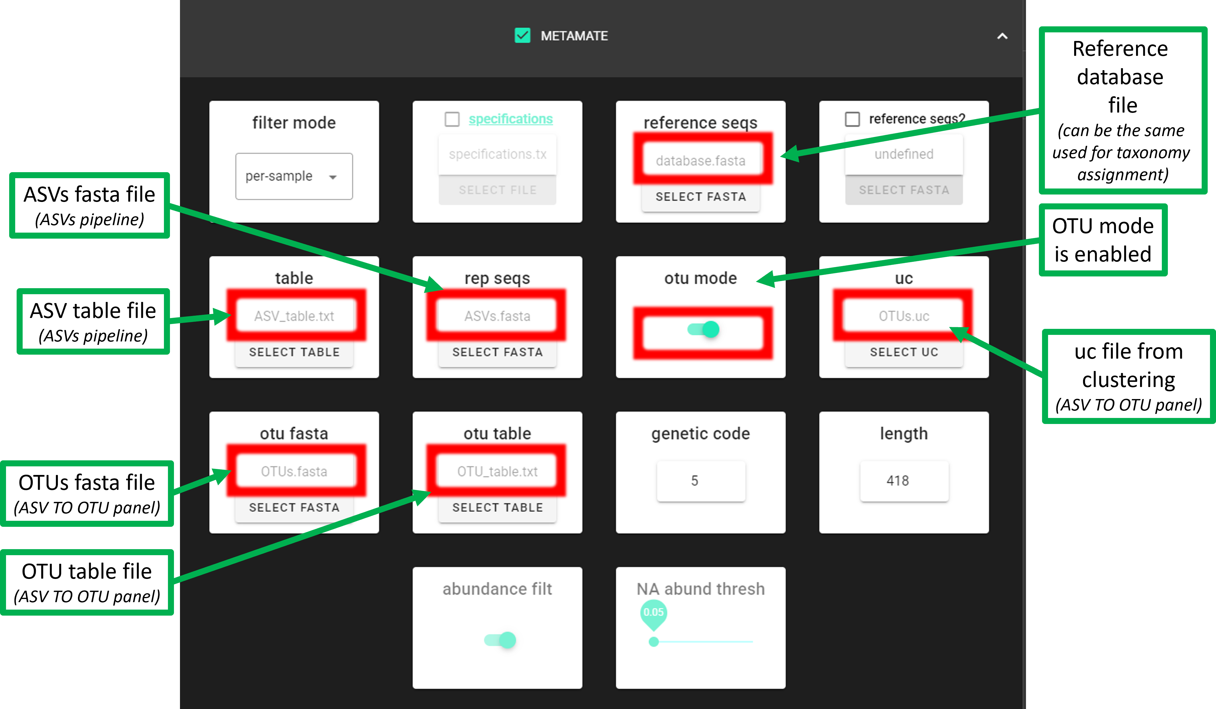
files needed for the OTU mode

In addition to the OTU table and OTUs.fasta files, ASVs.fasta and ASV table are also needed for the OTU mode. Therefore, OTU mode can be used when you have performed ASVs pipeline (DADA2 or UNOISE) and then clustered ASVs to OTUs (Postprocessing -> ‘ASV TO OTU’).

If you do not have the ASVs.fasta and ASV table files (that is, you have performed OTUs pipeline), then run metaMATE with otu mode disabled. However, note that metaMETA will then work only with the representative sequences of OTUs.

If planning to use LULU POST-CLUSTERING, then perform this after applying metaMATE (because after LULU, the uc file from clustering is not anymore compatible with OTU table, and thus metaMATE cannot work with post-clustered OTUs).

memory (RAM) usage

if a reference database (reference seqs) is very large, then the process may require a lot of RAM. If you receive an error message “.ERROR: BBMap alignment produced no matches and a memory error was detected”, then you may need to increase the memory (RAM) allocated to Docker and or close other applications that are using a lot of RAM.

Outputs

Outputs are in metamate_out directory:

Output directory
when global filter is used
*.metaMATE.txt	filtered feature (ASV/OTU) table
*metaMATE.fasta	retained features (ASVs/OTUs)
*metaMATE.list	list of IDs of retained features
sequence_counts.txt	a text file containing the number of sequences per sample
otu_summary.csv [if `otu mode` = TRUE ]	summary of ASV_Status and OTU_Status. Authentic = feature that perfectly matched the reference sequence Non-Authentic = feature that did not pass the genetic code translation or length filter Unclassified = feature that was not classified as Authentic or Non-Authentic
`metaMATE-find`/ passes_and_fails.txt	list of features with refpass, lenghtfails and stopfails. refpass = feature that perfectly matched the reference sequence lenghtfails = feature did not pass the length filter stopfails = feature did not pass the stop codon filter
`metaMATE-find`/results.csv	metaMATE find results file. See metaMATE documentation for more info about the results file
`metaMATE-find`/ selected_result_index.txt	contains the selected resultindex for results.csv file for metaMATE-dump
when per-sample filter is used
*.metaMATE.txt	filtered feature (ASV/OTU) table
*metaMATE.fasta	filtered features (ASVs/OTUs)
passes_and_fails.txt	list of features with refpass, lenghtfails and stopfails. refpass = feature that perfectly matched the reference sequence lenghtfails = feature did not pass the length filter stopfails = feature did not pass the stop codon filter
filter-adaptive_summary.csv	summary of applied thresholds, authentic and non-authentic features for each sample
otu_summary.csv [if `otu mode` = TRUE ]	summary of ASV_Status and OTU_Status. Authentic = feature that perfectly matched the reference sequence Non-Authentic = feature that did not pass the genetic code translation or length filter Unclassified = feature that was not classified as Authentic or Non-Authentic

More detailed information about the output files can be found in the metaMATE github repository.

ORF-Finder

Filter out putative pseudogenes (NUMTs) from protein coding amplicon dataset (such as COI, rbcL) using NCBI’s ORFfinder (Sayers et al 2022). This process translates sequences to open reading frames (ORFs) and retaines the longest ORF per sequence if the length of the ORF is between the specified range of min length and max length.

Check and specify the min length and max length of the expected amplicon sequence and genetic code (based on the target organism; 5 = invertebrate mitochondrial code. Use 1 for rbcL. Specify values from 1 to 33.

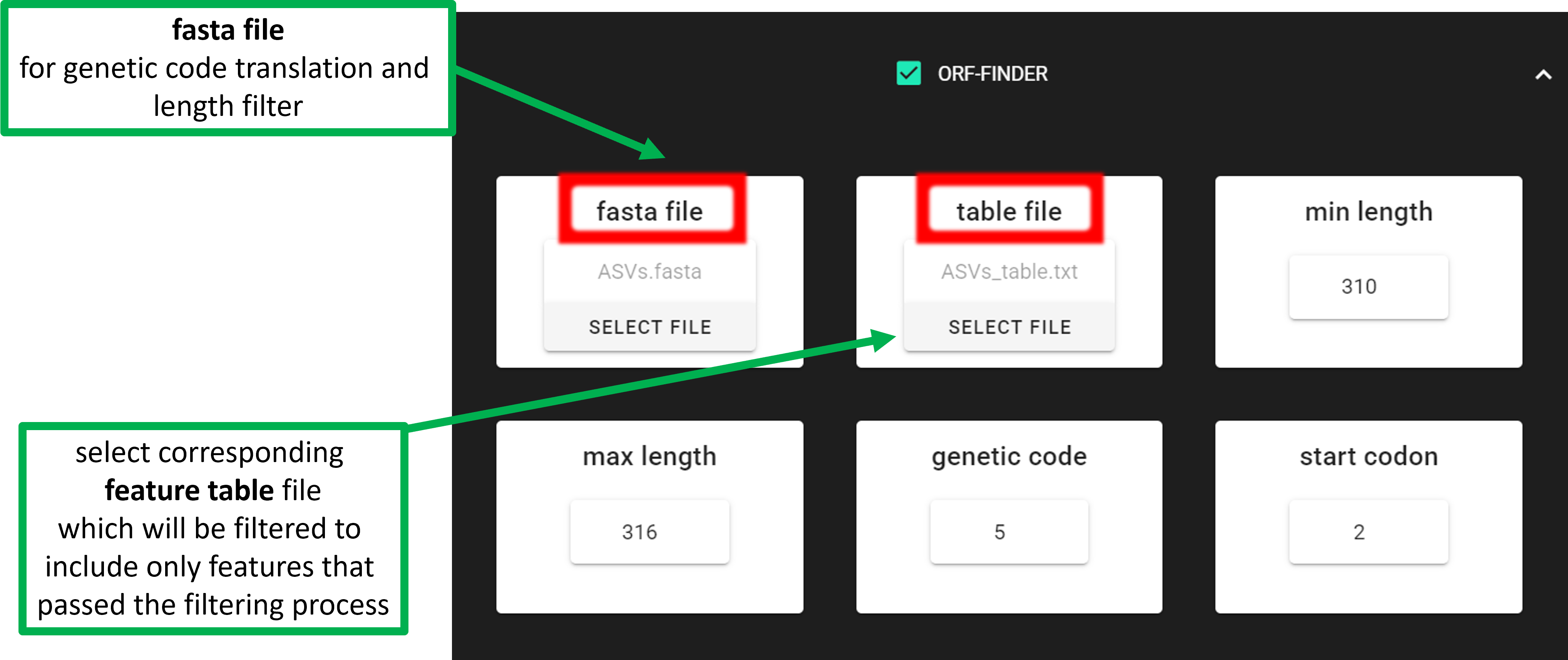
In the above example, the target COI amplicon is 313 bp, and target taxa are invertebrates. Therefore, the genetic code is 5. By specifying min length = 310 and max length = 316, we are allowing length variation up to one codon (±3 bp) around the target amplicon length. Only input sequences with open reading frames (ORFs) that are within the specified length range are kept.

Input data

The input table format; can contain “Sequence” column:

ASV	Sequence	Sample_1	Sample_2	Sample_3	…
ASV_1	ATGCTGATC…	0	200	320	…
ASV_2	ATGCTGATC…	99	200	222	…
ASV_3	ATGCTGATC…	10	34	3	…

To START

To START, specify working directory under SELECT WORKDIR (outputs will be written here), but the following requests about Sequence files extension and Sequencing read types do not matter here, just click ‘Confirm’.

Settings

Setting	Tooltip
`fasta file`	select fasta formatted sequence file containing your OTU/ASV reads. Sequence IDs must NOT contain underlines ‘_’ [fasta file must be in the SELECT WORKDIR directory]
`table file`	select features table file that contains corresponding features (OTUs/ASVs) to the fasta file [file must be in the SELECT WORKDIR directory]
`min length`	minimum length of an output sequence.
`max length`	maximum length of an output sequence.
`genetic code`	set the genetic code of the expected amplicon sequence.
`start codon`	translation table used to translate input sequences when checking for stop codons.
`ignore nested`	ignore nested open reading frames (completely placed within another).
`strand`	output open reading frames (ORFs) on specified strand only. Both = search also reverse complement.

Outputs

The outputs are in the selected working directory (ORF_filtered):

Output file	Description
`*_ORFs.fasta`	fasta file of sequences that passed ORF-finder
`*_ORFs.list.txt`	list of sequences that passed ORF-finder
`*.ORFs.txt`	filtered feature table containing only sequences that passed ORF-finder
`notORFs/*_notORFs.fasta`	fasta file of sequences that did not pass ORF-finder
`notORFs/*_notORFs.list.txt`	list of sequences that did not pass ORF-finder

BlasCh

False positive chimera detection and recovery module. BlasCh (BLAST-based Chimera detection) uses BLAST alignment analysis to identify, classify, and recover sequences that were incorrectly flagged as chimeric during initial chimera detection steps.

Important

Workflow compatibility requirements:

Currently, BlasCh is not a part of a pre-compiled pipeline - it is a standalone post-processing tool
Must be used after chimera filtering has been completed: after chimera filtering is finished → run BlasCh → run clustering etc…
If a nonchimeric/ folder is present in the working directory, BlasCh automatically merges rescued sequences with the pre-existing non-chimeric sequences into BlasCh_out/nonchimeric+rescued_reads/

BlasCh employs a BLAST-based approach to re-evaluate chimeric sequences through multiple analysis steps:

Database Creation: Creates BLAST databases from both sample FASTA files (self-databases) and reference sequences
BLAST Analysis: Performs nucleotide BLAST searches against both self-databases and reference database
Hit Analysis: Examines BLAST alignments for multiple High-scoring Segment Pairs (HSPs), taxonomic diversity, and alignment quality
Classification: Applies multi-tier thresholds to classify sequences into distinct categories based on identity and coverage metrics
Recovery: Rescues sequences that meet quality criteria for inclusion in downstream analyses

The module implements smart rerun capabilities, automatically detecting and reusing existing BLAST XML files to enable parameter optimization without re-running computationally expensive BLAST searches.

Input data are sequences (putative chimeric sequences) in FASTA format (.chimeras.fasta, .chimeras.fa, .chimeras.fas files) and a reference database (FASTA file or existing BLAST database).

Optionally, a nonchimeric/ subfolder may be placed in the working directory, containing pre-existing non-chimeric sequences per sample in basename.fasta format (same naming convention as the self-database source files). When present, BlasCh merges those sequences with the recovered *_non_chimeric.fasta reads into a combined BlasCh_out/nonchimeric+rescued_reads/ folder.

Important

File organization requirements:

Input chimera files (.chimeras.fasta / .chimeras.fa / .chimeras.fas) must be placed directly in the working directory
Sample FASTA files (the per-sample sequences before chimera filtering) must be placed in a subfolder named self_database/ inside the working directory — BlasCh reads them from there to build per-sample BLAST self-databases
Reference database files must be stored in a separate directory from the working directory to avoid conflicts
Do not mix reference database files with input chimera files or self-database FASTAs

Expected input folder structure:

workdir/                         ← SELECT WORKDIR in PipeCraft2
├── sample1.chimeras.fasta       ← chimeric sequences output from denoiser
├── sample2.chimeras.fasta       ← (placed directly in workdir)
├── self_database/               ← original per-sample FASTAs (before chimera filtering)
│   ├── sample1.fasta
│   └── sample2.fasta
├── nonchimeric/                 ← (optional) non-chimeric reads per sample (after chimera filtering)
│   ├── sample1.fasta
│   └── sample2.fasta
└── /path/to/reference_db/       ← reference database in a SEPARATE location
    └── reference.fasta

Settings

Setting	Tooltip
`reference_db`	path to reference database (FASTA file or existing BLAST database). Required - must be provided and stored in separate folder from input files
`high_identity_threshold`	identity threshold for high-quality matches (default: 99.0%)
`high_coverage_threshold`	coverage threshold for high-quality matches (default: 99.0%)
`borderline_identity_threshold`	identity threshold for borderline recovery (default: 80.0%)
`borderline_coverage_threshold`	coverage threshold for borderline recovery (default: 89.0%)

Outputs

Outputs are in BlasCh_out directory:

Output directory	`BlasCh_out`
RESCUED SEQUENCES (main results)
`nonchimeric`/`*_non_chimeric.fasta`	recovered non-chimeric sequences (high confidence rescue)
`borderline`/`*_borderline.fasta`	borderline sequences (moderate confidence rescue)
`nonchimeric+rescued_reads`/`*.fasta`	merged file per sample: input `nonchimeric/` sequences + BlasCh-recovered `*_non_chimeric` sequences
SUMMARY AND REPORTS
chimera_recovery_report.txt	summary statistics and classification results
README.txt	documentation of analysis parameters and results
DETAILED ANALYSIS RESULTS
`detailed_results`/`*_multiple_alignments.fasta`	sequences with multiple HSPs and low coverage
`detailed_results`/`*_sequence_details.csv`	detailed classification results for each sequence
TECHNICAL FILES
`xml`/blast_results.zip	compressed BLAST XML output files (can be used for reanalysis with different thresholds)

Folder organization explanation:

Rescued Sequences: The non_chimeric and borderline folders contain sequences that can be included in downstream analyses
Merged Output: The nonchimeric+rescued_reads folder (created only when a nonchimeric/ input folder is provided) combines the pre-existing non-chimeric sequences with BlasCh-recovered sequences per sample, ready for direct use in clustering or downstream analyses
Detailed Results: The detailed_results folder contains sequences that remain excluded along with analysis details
Summary Files: Report files provide overview statistics and complete documentation of the analysis
Technical Files: Compressed XML files allow reanalysis with different parameters without re-running BLAST

Detailed classification logic

BlasCh uses multi-tier classification system with the following decision tree:

Multiple alignments: Sequences with multiple HSPs in the first non-self BLAST alignment and ≤85% coverage → classified as multiple alignments
Self-hits only: Sequences that only match to their own sample without reference database matches → confirmed chimeric
High-Quality matches: Identity ≥threshold AND coverage ≥threshold against reference database → rescued as non-chimeric
Borderline recovery: Identity ≥threshold AND coverage ≥threshold against reference database → rescued as non-chimeric
Taxonomic diversity: Multiple different taxonomies in top hits without meeting quality thresholds → confirmed chimeric

Smart rerun capability:

Automatically detects existing BLAST XML files from previous runs
Extracts XML files from compressed archives when needed
Skips database creation and BLAST steps if XML files are complete
Enables testing different classification thresholds without re-running BLAST
Handles mixed scenarios (some samples have XML, others don’t)

Expected Results:

Rescued sequences (non-chimeric and borderline) can be included in downstream analyses
Detailed analysis results provide transparency about why certain sequences were confirmed as chimeric
CSV reports contain per-sequence classification details and summary statistics
Documentation ensures reproducibility and parameter tracking

Post-BlasCh Workflow:

Merge rescued sequences with original non-chimeric sequences from each sample
- Automatic: place a nonchimeric/ folder (containing basename.fasta files) in the working directory before running BlasCh. The merged output will be written to BlasCh_out/nonchimeric+rescued_reads/ automatically.
- Manual: combine non_chimeric/*_non_chimeric.fasta files with the corresponding per-sample non-chimeric sequences yourself.
Run clustering manually on the combined sequence sets (use nonchimeric+rescued_reads/ if the automatic merge was performed)
Proceed with downstream analyses using the updated sequence data
Document which sequences were rescued for transparency in results

Note

BlasCh automatically detects .chimeras files with various extensions (.fasta, .fa, .fas) in the working directory and creates self-databases from available sample FASTA files. Original sample files are prioritized over .chimeras files for database creation.

Warning

Important usage notes:

Ensure chimera detection has been run prior to BlasCh analysis
Reference database must be provided and in FASTA format or valid BLAST database format
Reference database files must be stored in a separate directory from input files

DEICODE 

DEICODE (Martino et al., 2019) is used to perform beta diversity analysis by applying robust Aitchison PCA on the OTU/ASV table. To consider the compositional nature of data, it preprocesses data with rCLR transformation (centered log-ratio on only non-zero values, without adding pseudo count). As a second step, it performs dimensionality reduction of the data using robust PCA (also applied only to the non-zero values of the data), where sparse data are handled through matrix completion.

Additional information:

Input data

Input data is tab delimited OTU table and optionally subset of OTU ids to generate results also for the selected subset (see input examples below).

Example of input table (tab delimited text file):

OTU_id	sample1	sample2	sample3	sample4
00fc1569196587dde	106	271	584	20
02d84ed0175c2c79e	81	44	88	14
0407ee3bd15ca7206	3	4	3	0
042e5f0b5e38dff09	20	83	131	4
07411b848fcda497f	1	0	2	0
07e7806a732c67ef0	18	22	83	7
0836d270877aed22c	1	1	0	0
0aa6e7da5819c1197	1	4	5	0
0c1c219a4756bb729	18	17	40	7

Example of input subset_IDs:

07411b848fcda497f
042e5f0b5e38dff09
0836d270877aed22c
0c1c219a4756bb729
...

To START

To START, specify working directory under SELECT WORKDIR (outputs will be written here), but the following requests about Sequence files extension and Sequencing read types do not matter here, just click ‘Confirm’.

Settings

Setting	Tooltip
`table`	select OTU/ASV table. If no file is selected, then PipeCraft will look OTU_table.txt or ASV_table.txt in the working directory. See OTU table example below
`subset_IDs` (optional)	select list of OTU/ASV IDs for analysing a subset from the full table see subset_IDs file example below
`min_otu_reads`	cutoff for reads per OTU/ASV. OTUs/ASVs with lower reads then specified cutoff will be excluded from the analysis
`min_sample_reads`	cutoff for reads per sample. Samples with lower reads then specified cutoff will be excluded from the analysis

Outputs

Outputs are in DEICODE_out directory:

Output directory `DEICODE_out`
otutab.biom	full OTU table in BIOM format
rclr_subset.tsv	rCLR-transformed subset of OTU table *
`full`/distance-matrix.tsv	distance matrix between the samples, based on full OTU table
`full`/ordination.txt	ordination scores for samples and OTUs, based on full OTU table
`full`/rclr.tsv	rCLR-transformed OTU table
`subs`/distance-matrix.tsv	distance matrix between the samples, based on a subset of OTU table *
`subs`/ordination.txt	ordination scores for samples and OTUs, based a subset of OTU table *
* files are present only if ‘subset_IDs’ variable was specified

PERMANOVA and PERMDISP example using the robust Aitchison distance

library(vegan)

## Load distance matrix
dd <- read.table(file = "distance-matrix.tsv")

## You will also need to load the sample metadata
## However, for this example we will create a dummy data
meta <- data.frame(
  SampleID = rownames(dd),
  TestData = rep(c("A", "B", "C"), each = ceiling(nrow(dd)/3))[1:nrow(dd)])

## NB! Ensure that samples in distance matrix and metadata are in the same order
meta <- meta[ match(x = meta$SampleID, table = rownames(dd)), ]

## Convert distance matrix into 'dist' class
dd <- as.dist(dd)

## Run PERMANOVA
adon <- adonis2(formula = dd ~ TestData, data = meta, permutations = 1000)
adon

## Run PERMDISP
permdisp <- betadisper(dd, meta$TestData)
plot(permdisp)

Example of plotting the ordination scores

library(ggplot2)

## Load ordination scores
ord <- readLines("ordination.txt")

## Skip PCA summary
ord <- ord[ 8:length(ord) ]

## Break the data into sample and species scores
breaks <- which(! nzchar(ord))
ord <- ord[1:(breaks[2]-1)]               # Skip biplot scores
ord_sp <- ord[1:(breaks[1]-1)]            # species scores
ord_sm <- ord[(breaks[1]+2):length(ord)]  # sample scores

## Convert scores to data.frames
ord_sp <- as.data.frame( do.call(rbind, strsplit(x = ord_sp, split = "\t")) )
colnames(ord_sp) <- c("OTU_ID", paste0("PC", 1:(ncol(ord_sp)-1)))

ord_sm <- as.data.frame( do.call(rbind, strsplit(x = ord_sm, split = "\t")) )
colnames(ord_sm) <- c("Sample_ID", paste0("PC", 1:(ncol(ord_sm)-1)))

## Convert PCA to numbers
ord_sp[colnames(ord_sp)[-1]] <- sapply(ord_sp[colnames(ord_sp)[-1]], as.numeric)
ord_sm[colnames(ord_sm)[-1]] <- sapply(ord_sm[colnames(ord_sm)[-1]], as.numeric)

## At this step, sample and OTU metadata could be added to the data.frame

## Example plot
ggplot(data = ord_sm, aes(x = PC1, y = PC2)) + geom_point()

Post-processing tools 

Filter tag-jumps

Input data

Settings

Outputs

ASV to OTU

Input data

Settings

Outputs

LULU post-clustering

Input data

Settings

Outputs

DADA2 collapse ASVs

Input data

Settings

Outputs

metaMATE

Input data

Settings

OTU mode

Outputs

ORF-Finder

Input data

Settings

Outputs

BlasCh

Settings

Outputs

Detailed classification logic

DEICODE

Input data

Settings

Outputs

PERMANOVA and PERMDISP example using the robust Aitchison distance

DEICODE 