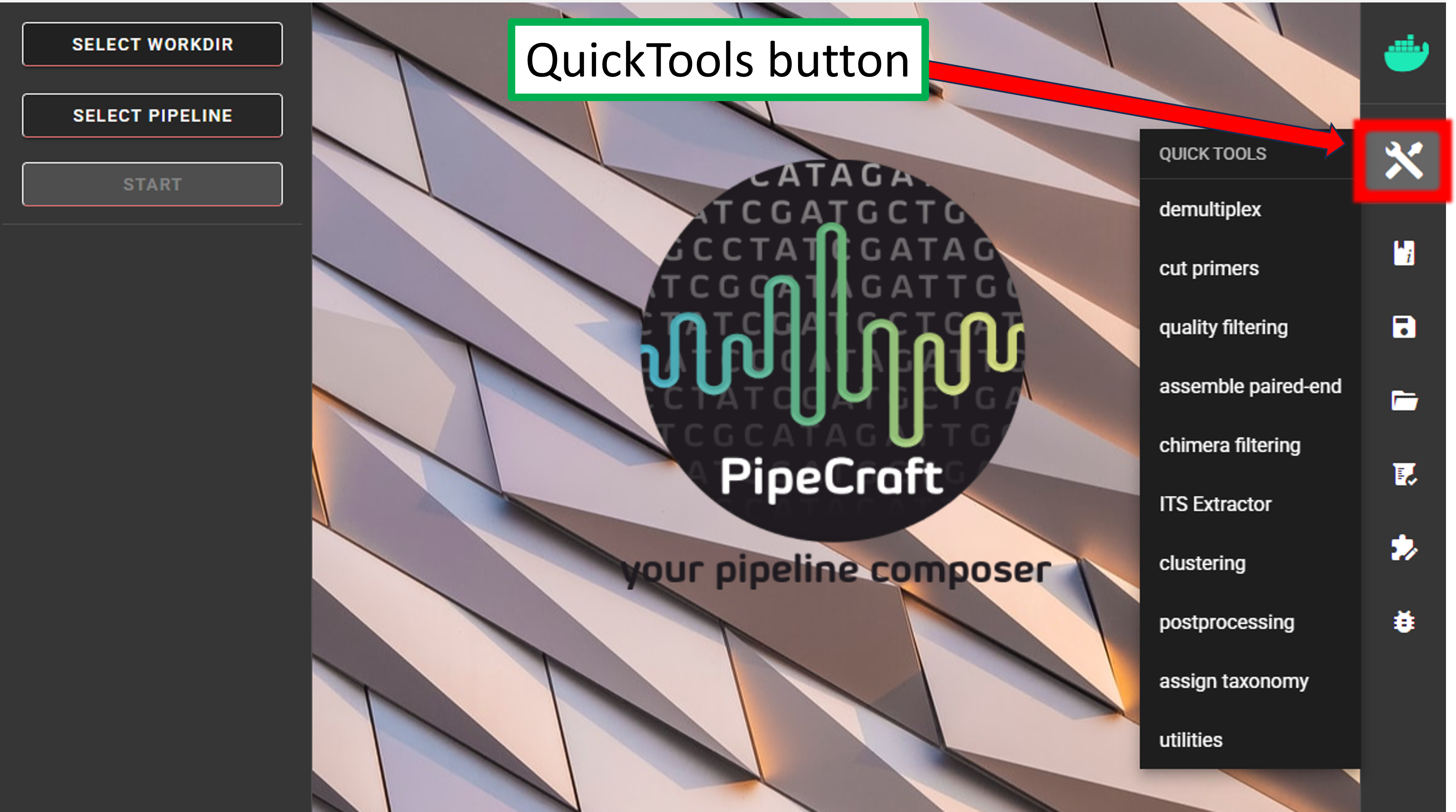
Individual steps (Quick Tools) 

QuickTools provide a list of processes that can be used to perform individual steps of the analysis (i.e., perform a custom pipeline). They are accessed by pressing the Quick Tools button on the right-ribbon interface.

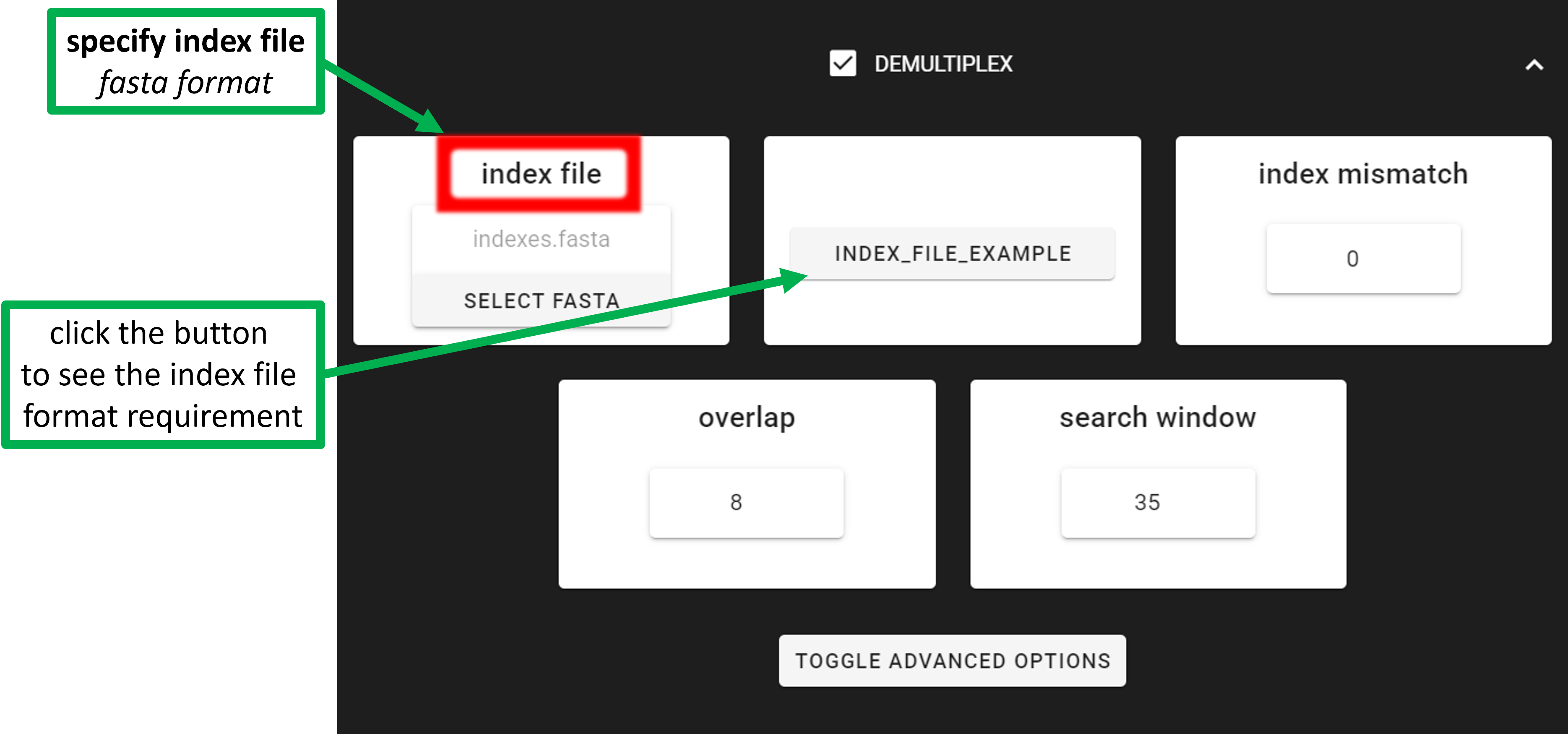
DEMULTIPLEXING

If the data is multiplexed, the first step would be demultiplexing. PipeCraft2 wraps cutadapt (Martin 2011) to perform demultiplexing. Demultiplexing is done based on the user specified indexes file, which includes molecular identifier sequences (so-called indexes/tags/barcodes) per sample.

Note that reverse complementary matches will also be searched, so if your data consists of amplicons that are both 5’-3’ and 3’-5’ oriented, then this is accounted for automatically.

Note

Heterogenity spacers or any redundant base pairs attached to index sequences do not affect demultiplexing. Indexes are trimmed from the best matching position.

Input data

Input fastq/fasta file must be in the working directory (specified with SELECT WORKDIR button).

my_multiplexed_fastq_file/     --> SELECT THIS FOLDER AS WORKING DIRECTORY
├── data_multiplexed.fastq.gz *[ONE fastq or fasta file in the WORKDIR for demultiplexing!]*
└── indexes.fasta

Index file location is specified with index file button, thus can be anywhere in the system (as long as the file path does not contain non-ASCII symbols).

Supported file formats

Supported file formats: paired-end or single-end fastq/fasta file for demultiplexing; and indexes file must be fasta format (see below for example).

Download example set here for trying demultiplexing and unzip it.

Settings

Setting	Tooltip
`index file`	select your fasta formatted indexes file for demultiplexing (see guide here), where fasta headers are sample names, and sequences are sample specific index or index combination
`index mismatch`	allowed mismatches during the index search
`overlap`	number of overlap bases with the index. Recommended overlap is the maximum length of the index for confident sequence assignments to samples
`search window`	the index search window size. The default 35 means that the forward index is searched among the first 35 bp and the reverse index among the last 35 bp. This search restriction prevents random index matches in the middle of the sequence
`no indels`	do not allow insertions or deletions is primer search. Mismatches are the only type of errors accounted in the error rate parameter
`min length`	minimum length of the output sequence

Outputs

Outputs are fastq/fasta files per sample in demultiplexed_out directory. Indexes are truncated from the sequences. Paired-end samples get .R1 and .R2 read identifiers. unknown.fastq file contain sequences where specified index combinations were not found.

Note

When using paired indexes, then sequences with all possible index combinations will be outputted to ‘unnamed_index_combinations’ dir. That means, if, for example, your sample_1 is indexed with indexFwd_1-indexRev_1 and sample_2 with indexFwd_2-indexRev_2, then files with indexFwd_1-indexRev_2 and indexFwd_2-indexRev_1 are also written (although latter index combinations were not used in the lab to index any sample [i.e. represent tag-switches]). Simply remove those files if not needed or use to estimate tag-switching error if relevant.

Indexes file example (fasta formatted)

Note

Only IUPAC codes are allowed in the sequences. Avoid using ‘.’ in the sample names (e.g. instead of sample.1, use sample_1)

Demultiplexing using single indexes:

>sample1

AGCTGCACCTAA

>sample2

AGCTGTCAAGCT

>sample3

AGCTTCGACAGT

>sample4

AGGCTCCATGTA

>sample5

AGGCTTACGTGT

>sample6

AGGTACGCAATT

Demultiplexing using paired (dual) indexes:

Important

IMPORTANT! The reverse indexes must be in the 3’-5’ orientation in the indexes file when doing demultiplexing in PipeCraft, because reverse indexes are automatically oriented to 5’-3’ under the hood. This facilitates the simple copy-paste of the indexes from the lab protocol. Therefore, if you have pre-compliled indexes file, so, that you have reverse indexes already reverse-comlemented (5’-3’ orientation), then the demultiplexing will fail (all will be unknown.fastq).

>sample1
AGCTGCACCTAA…AGCTGCACCTAA
>sample2
AGCTGTCAAGCT…AGCTGTCAAGCT
>sample3
AGCTTCGACAGT…AGCTTCGACAGT
>sample4
AGGCTCCATGTA…AGGCTCCATGTA
>sample5
AGGCTTACGTGT…AGGCTTACGTGT
>sample6
AGGTACGCAATT…AGGTACGCAATT

Note

Anchored indexes (https://cutadapt.readthedocs.io/en/stable/guide.html#anchored-5adapters) with ^ symbol are not supported in PipeCraft demultiplex GUI panel. Instead, specify search window = 0.

DO NOT USE, e.g.

>sample1
^AGCTGCACCTAA

>sample1
^AGCTGCACCTAA…AGCTGCACCTAA

How to compose indexes.fasta

In Excel (or any alternative program); first column represents sample names, second (and third) column represent indexes (or index combinations) per sample:

Example of single-end indexes

sample1    AGCTGCACCTAA
sample2    AGCTGTCAAGCT
sample3    AGCTTCGACAGT
sample4    AGGCTCCATGTA
sample5    AGGCTTACGTGT
sample6    AGGTACGCAATT

Example of paired indexes

sample1    AGCTGCACCTAA    AGCTGCACCTAA
sample2    AGCTGTCAAGCT    AGCTGTCAAGCT
sample3    AGCTTCGACAGT    AGCTTCGACAGT
sample4    AGGCTCCATGTA    AGGCTCCATGTA
sample5    AGGCTTACGTGT    AGGCTTACGTGT
sample6    AGGTACGCAATT    AGGTACGCAATT

Copy those two (or three) columns to text editor that support regular expressions, such as NotePad++ or Sublime Text.

single-end indexes:
1. Open ‘find & replace’ Find ^ (which denotes the beginning of each line). Replace with > (and DELETE THE LAST > in the beginning of empty row).
2. Find \t (which denotes tab). Replace with \n (which denotes the new line).
  
  FASTA FORMATTED (single-end indexes) indexes.fasta file is ready; SAVE the file.
Paired indexes:
1. Open ‘find & replace’: Find ^ (denotes the beginning of each line); replace with > (and DELETE THE LAST > in the beginning of empty row).
2. Find .*\K\t (which captures the second tab); replace with … (to mark the linked paired-indexes).
3. Find \t (denotes the tab); replace with \n (denotes the new line).
  
  FASTA FORMATTED (paired indexes) indexes.fasta file is ready; SAVE the file.

CUT PRIMERS

If the input data contains PCR primers (or e.g. adapters), these can be removed in the CUT PRIMERS panel. CUT PRIMERS processes relies on cutadapt (Martin 2011).

For generating OTUs or ASVs, it is recommended to truncate the primers from the reads Sequences where PCR primer strings were not detected are discarded by default (but stored in ‘untrimmed’ directory).

Reverse complementary search of the primers in the sequences is also performed. Thus, primers are clipped from both 5’-3’ and 3’-5’ oriented reads. However, note that paired-end reads will not be reoriented to 5’-3’ during this process, but single-end reads will be reoriented to 5’-3’.

When you may want to keep the primers

When you are working with ITS sequences and plan to use ITS Extractor to remove flanking primer binding regions from ITS1/ITS2/full ITS: if the ITS primer binding sites are very close to the ITS region (< 25 bp), then you may want to keep the primers for better detection of the 18S, 5.8S and/or 28S regions.

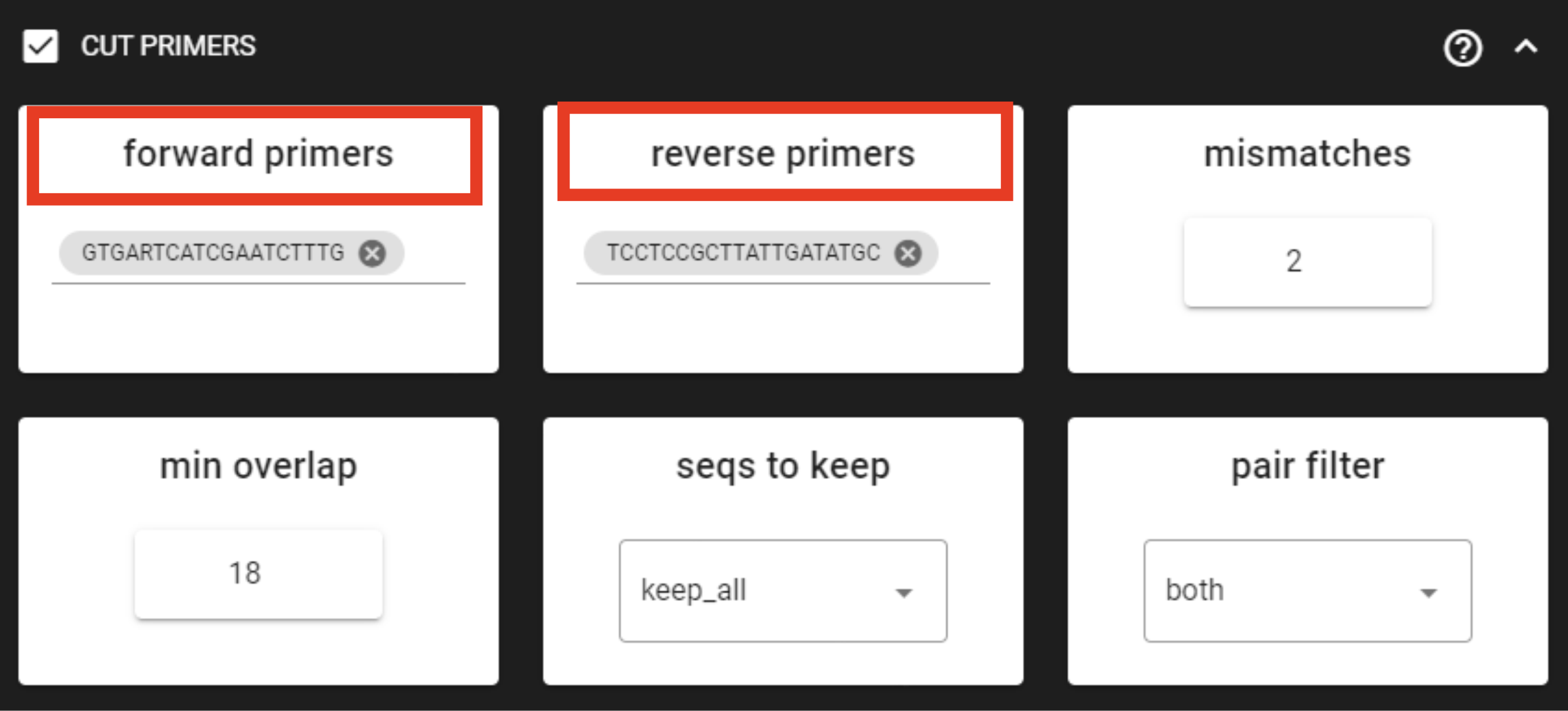
Example above: Forward primer has 19 bp and reverse 20 bp - to keep a bit of flexibility in the primer search, we are requesting the min overlap of 18 bp and are allowing maximum of 2 mismatches . Note that too low min overlap may lead to random matches.

Input data

Input fastq/fasta file(s) must be in the working directory (specified with SELECT WORKDIR button).

my_data/    --> SELECT THIS FOLDER AS WORKING DIRECTORY
├── sample1.fastq.gz
├── sample2.fastq.gz
├── sample3.fastq.gz
└── ...

Supported file formats

Supported file formats: paired-end or single-end fastq/fasta files.

When working with ITS sequences …

… and applying the ITSx step, then note that cutting primers process may be skipped, since those regions are removed in the ITS subregion extraction process.

Settings

Setting	Tooltip
`forward primers`	specify forward primer (5’-3’); IUPAC codes allowed; add up to 13 primers
`reverse primers`	specify reverse primer (3’-5’); IUPAC codes allowed; add up to 13 primers
`mismatches`	allowed mismatches in the primer search
`min overlap`	number of overlap bases with the primer sequence. Partial matches are allowed, but short matches may occur by chance, leading to erroneously clipped bases. Specifying higher overlap than the length of primer sequnce will still clip the primer (e.g. primer length is 22 bp, but overlap is specified as 25 - this does not affect the identification and clipping of the primer as long as the match is in the specified mismatch error range)
`seqs to keep`	keep sequences where at least one primer was found (fwd or rev); recommended when cutting primers from paired-end data (unassembled), when individual R1 or R2 read lengths are shorther than the expected amplicon length. ‘keep_only_linked’ = keep sequences if primers are found in both ends (fwd…rev); discards the read if both primers were not found in this read
`pair filter`	applies only for paired-end data. ‘both’, means that a read is discarded only if both, corresponding R1 and R2, reads do not contain primer strings (i.e. a read is kept if R1 contains primer string, but no primer string found in R2 read). Option ‘any’ discards the read if primers are not found in both, R1 and R2 reads
`no indels`	do not allow insertions or deletions is primer search. Mismatches are the only type of errors accounted in the error rate parameter

Note

For paired-end data, the seqs_to_keep option should be left as default (‘keep_all’). This will output sequences where at least one primer has been clipped. ‘keep_only_linked’ option outputs only sequences where both the forward and reverse primers are found (i.e. 5’-forward…reverse-3’). ‘keep_only_linked’ may be used for single-end data to keep only full-length amplicons.

Outputs

Outputs are fastq/fasta files in primersCut_out directory. Primers are truncated from the sequences. Sequences where primers were not found are stored in untrimmed directory.

QUALITY FILTERING

Quality filtering removes low-quality sequences before downstream analysis. Keeping only high-quality sequences prevents noisy data from creating erroneous OTUs/ASVs. Different tools implement quality filtering in slightly different ways, but the goal is the same: retain sequences that meet the specified threshold(s).

Before running quality filtering, it is best to inspect the sequence quality profiles to see where quality starts to decline and which trimming settings could be appropriate. Checkout the Inspect quality profiles section for a walkthrough of this step.

Input data

Input fastq file(s) must be in the working directory (specified with SELECT WORKDIR button).

 my_data/    --> SELECT THIS FOLDER AS WORKING DIRECTORY
├── sample1.fastq.gz
├── sample2.fastq.gz
├── sample3.fastq.gz
└── ...

Supported file formats

Supported file formats: paired-end or single-end fastq files.

Outputs

Outputs are quality filtered fastq files in qualFiltered_out directory.

Below lists the different quality filtering tools implemented in PipeCraft2.

vsearch 

Vsearch (fastq_filter function) filters reads by calculating the expected errors per read (maxee; sum of per-base error probabilities derived from Phred scores) and discards reads exceeding the threshold. In addition, reads can be removed based on ambiguous bases (maxNs) and length constraints (min length / max length), and optionally truncated to a fixed length (trunc length). Applying trunc length, strip_left and strip_right may be helpful to remove low-quality ends/starts of reads before filtering (maxee filtering is applied to the truncated reads).

vsearch setting	Tooltip
`maxee`	maximum number of expected errors per sequence (see here). Sequences with higher error rates will be discarded
`maxNs`	discard sequences with more than the specified number of Ns
`min length`	minimum length of the filtered output sequence
`trunc length`	truncate sequences to the specified length. Shorter sequences are discarded; thus if specified, check that ‘min length’ setting is lower than ‘trunc length’ (‘min length’ therefore has basically no effect) [empty field = no action taken]
`qmax`	specify the maximum quality score accepted when reading FASTQ files. The default is 41, which is usual for recent Sanger/Illumina 1.8+ files. For PacBio data use 50-93
`max length`	discard sequences with more than the specified number of bases. Note NOT be lower than ‘trunc length’ (otherwise all reads are discared) [empty field = no action taken] Note that if ‘trunc length’ setting is specified, then ‘min length’ SHOULD BE lower than ‘trunc length’ (otherwise all reads are discared)
`qmin`	the minimum quality score accepted for FASTQ files. The default is 0, which is usual for recent Sanger/Illumina 1.8+ files. Older formats may use scores between -5 and 2
`maxee rate`	discard sequences with more than the specified number of expected errors per base
`truncqual`	tuncate sequences starting from the first base with the specified base quality score value or lower (0 or empty field = no action taken)
`truncee`	truncate sequences so that their total expected error is not higher than the specified value (0 or empty field = no action taken)
`strip_left`	Default 0. The number of base pairs to remove from the start of each read
`strip_right`	Default 0. The number of nucleotides to remove from the end of each read

trimmomatic 

Trimmomatic

Trimmomatic trims and filters reads based on base-quality scores. The main trimming is performed with a sliding-window approach: Trimmomatic scans from the 5’ end and cuts the read once the mean quality in a window (window_size) drops below the threshold (required_quality). Optional additional steps remove low-quality bases at the start (leading_qual_threshold) and end (trailing_qual_threshold) of reads. Reads shorter than min_length after trimming are discarded.

trimmomatic setting	Tooltip
`window_size`	the number of bases to average base qualities. Starts scanning at the 5’-end of a sequence and trimms the read once the average required quality (required_qual) within the window size falls below the threshold
`required_quality`	the average quality required for selected window size
`min_length`	minimum length of the filtered output sequence
`leading_qual_threshold`	quality score threshold to remove low quality bases from the beginning of the read. As long as a base has a value below this threshold the base is removed and the next base will be investigated
`trailing_qual_threshold`	quality score threshold to remove low quality bases from the end of the read. As long as a base has a value below this threshold the base is removed and the next base will be investigated
`phred`	phred quality scored encoding. Default = 33. Use 64 if working with data from older Illumina (Solexa) machines

fastp 

fastp uses a sliding-window trimming approach, similar to Trimmomatic, (window_size + required_qual) to trim reads when local mean quality drops below the threshold. It scans reads from the 5’ end toward the 3’ end and trims the read from the first low-quality window onward (i.e. removes the low-quality 3’ tail). It additionally filters reads based on the fraction of low-quality bases (min_qual + min_qual_thresh), ambiguous bases (maxNs), minimum/maximum length (min_length / max_length).

fastp can also trim/remove reads affected by two common artifacts: polyG trimming removes artificial poly-G tails that can appear in some Illumina NextSeq/NovaSeq two-colour chemistry runs when signal drops and bases are miscalled as long runs of G. However, note that when clipping primers, those poly-G artifacts are removed, as the primer sequences are recorded before the signal drops. low-complexity filter removes reads dominated by repetitive/low-information sequence (e.g. homopolymers like AAAAAA or simple repeats).

fastp setting	Tooltip
`window_size`	the window size for calculating mean quality
`required_qual`	the mean quality requirement per sliding window (window_size)
`min_qual`	the quality value that a base is qualified. Default 15 means phred quality >=Q15 is qualified
`min_qual_thresh`	how many percents of bases are allowed to be unqualified (0-100)
`maxNs`	discard sequences with more than the specified number of Ns
`min_length`	minimum length of the filtered output sequence. Shorter sequences are discarded
`max_length`	reads longer than ‘max length’ will be discarded, default 0 means no limitation
`trunc_length`	truncate sequences to specified length. Shorter sequences are discarded; thus check that ‘min length’ setting is lower than ‘trunc length’
`aver_qual`	if one read’s average quality score <’aver_qual’, then this read/pair is discarded. Default 0 means no requirement
`low_complexity_filter`	enables low complexity filter and specify the threshold for low complexity filter. The complexity is defined as the percentage of base that is different from its next base (base[i] != base[i+1]). E.g. vaule 30 means then 30% complexity is required. Not specified = filter not applied

DADA2 (‘filterAndTrim’ function)

DADA2 (filterAndTrim function) filters reads based on expected errors (maxEE; same as vsearch) and ambiguous bases (maxN). It also allows for truncation of reads at the first instance of a quality score less than or equal to truncQ (applied to both R1 and R2 reads). Reads shorter than minLen after truncation are discarded. truncLen / truncLen_R2 options truncate reads to a fixed number of bases before maxEE filtering. trimLeft and trimRight options remove bases from the start and end of the reads, respectively. These options are useful to remove low-quality ends of reads before filtering.

DADA2 setting	Tooltip
`maxEE`	discard sequences with more than the specified number of expected errors
`maxN`	discard sequences with more than the specified number of N’s (ambiguous bases)
`minLen`	remove reads with length less than minLen. minLen is enforced after all other trimming and truncation
`truncQ`	truncate reads at the first instance of a quality score less than or equal to truncQ
`truncLen`	truncate reads after truncLen bases (applies to R1 reads when working with paired-end data). Reads shorter than this are discarded. Explore quality profiles (with QualityCheck module) and see whether poor quality ends needs to be truncated
`truncLen_R2`	applies only for paired-end data. Truncate R2 reads after truncLen bases. Reads shorter than this are discarded. Explore quality profiles (with QualityCheck module) and see whether poor quality ends needs to truncated
`maxLen`	remove reads with length greater than maxLen. maxLen is enforced on the raw reads. In dada2, the default = Inf, but here set as 9999
`minQ`	after truncation, reads contain a quality score below minQ will be discarded
`matchIDs`	applies only for paired-end data. If TRUE, then double-checking (with seqkit pair) that only paired reads that share ids are outputted
`trimLeft`	Default 0. The number of base pairs to remove from the start of each read
`trimRight`	Default 0. The number of nucleotides to remove from the end of each read

ASSEMBLE PAIRED-END reads

Assemble/merge paired-end reads (such as those from Illumina or MGI-Tech platforms) into a single sequence. This is done to reconstruct the full amplicon (or a longer contiguous region) from the forward (R1) and reverse (R2) reads when they overlap. Merging can improve accuracy in the overlap region because base conflicts are resolved using the quality scores. Assembling corresponding paired reads produces one read for downstream steps.

Assembly is not needed when you already have single-end data (e.g., already assembled, or PacBio data), when reads do not overlap (insert too long), or when you intentionally want to work with only R1 reads.

Input data

Input fastq file(s) must be in the working directory (specified with SELECT WORKDIR button).

 my_data/    --> SELECT THIS FOLDER AS WORKING DIRECTORY
├── sample1.R1.fastq.gz
├── sample1.R2.fastq.gz
├── sample2.R1.fastq.gz
├── sample2.R2.fastq.gz
├── sample3.R1.fastq.gz
├── sample3.R2.fastq.gz
├── sample4.R1.fastq.gz
├── sample4.R2.fastq.gz
└── ...

Supported file formats

Supported file formats:
paired-end fastq files, with R1 and R2 read identifiers (NOT just _1 and _2 suffixes, e.g. sample_L001_1.fastq and sample_L001_2.fastq).
File names may not contain R1/R2 strings.

Outputs

Outputs are assembled reads in assembled_out directory.

Below lists the different assembly tools implemented in PipeCraft2.

vsearch 

vsearch (–fastq_mergepairs function) merges paired-end reads based on overlap between the reads. The best-supported overlap is accepted only if it meets the spacified constraints (e.g., min_overlap and max_diffs). In the overlap region, base conflicts are resolved using the read quality scores (higher-quality base is preferred).

include_only_R1 represents additional in-built option in PipeCraft. If TRUE, unassembled R1 reads will be included to the set of assembled reads per sample. This may be relevant when working with e.g. ITS2 sequences, because the ITS2 region in some taxa is too long for paired-end assembly using short-read sequencing technology. Therefore longer ITS2 sequences are discarded completely after the assembly process. Thus, including also unassembled R1 reads (include_only_R1 = TRUE), partial ITS2 sequences for these taxa will be represented in the final output. But when using ITSx, keep only_full = FALSE and include partial = 50.

Setting	Tooltip
`min overlap`	minimum overlap between the merged reads
`min length`	minimum length of the merged sequence
`allow merge stagger`	when TRUE, vsearch will also attempt to merge staggered read pairs (pairs with an overhang rather than a clean overlap). This can occur when the insert/fragment is very short relative to the sequencing run. In that situation, after reverse-complementing R2 the reads can “pass” each other, so one read extends beyond the start of the other (an overhang). Enabling this option allows such short-insert pairs to be merged. Short inserts often come with adapter read-through; adapter/primer trimming helps, but very short inserts can still occur, so this option can be useful.
`include only R1`	Include unassembled R1 reads to the set of assembled reads per sample. This may be relevant when working with e.g. ITS2 sequences, because the ITS2 region in some taxa is too long for assembly, therefore discarded completely after assembly process. Thus, including also unassembled R1 reads, partial ITS2 sequences for these taxa will be represented in the final output
`max diffs`	the maximum number of non-matching nucleotides allowed in the overlap region
`max Ns`	discard sequences with more than the specified number of Ns
`max length`	maximum length of the merged sequence
`keep disjoined`	output reads that were not merged into separate FASTQ files
`fastq qmax`	maximum quality score accepted when reading FASTQ files. The default is 41, which is usual for recent Sanger/Illumina 1.8+ files

DADA2 

DADA2 (mergePairs function) merges paired-end reads based on overlap between the reads. It allows for trimming of overhangs in the alignment between the forwards and reverse read, and concatenation of the forward and reverse-complemented reverse read with a spacer of 10 Ns.

Important

Here, dada2 will perform also denoising (function ‘dada’) before assembling paired-end data. Because of that, input sequences (in fastq format) must consist of only A/T/C/Gs (no ambiguous bases (Ns)); therefore apply on quality-filtered reads. Due to denoising, this process takes longer compared with just merging paired-end reads.

Here, the output are all merged R1 and R2 reads in denoised_assembled.dada2 directory. As DADA2 denoising produces ASVs, then merged ASVs per samples are in the denoised_assembled.dada2/merged_ASVs directory.

Setting	Tooltip
`minOverlap`	the minimum length of the overlap required for merging the forward and reverse reads
`maxMismatch`	the maximum mismatches allowed in the overlap region
`trimOverhang`	if TRUE, overhangs in the alignment between the forwards and reverse read are trimmed off. Overhangs are when the reverse read extends past the start of the forward read, and vice-versa, as can happen when reads are longer than the amplicon and read into the other-direction primer region
`justConcatenate`	if TRUE, the forward and reverse-complemented reverse read are concatenated rather than merged, with a NNNNNNNNNN (10 Ns) spacer inserted between them
`errorEstFun`	denoising setting. DADA2 errorEstimationFunction: ‘loessErrfun’ for Illumina data; ‘PacBioErrfun’ for PacBio data
`nbases`	denoising setting. The minimum number of bases to use for error rate estimation. Default is 1e8 (100 million bases)
`randomize`	denoising setting. Default = TRUE. If TRUE, samples are picked at random from those provided. If FALSE, samples are picked in the order they are provided until enough reads are obtained.
`pool`	denoising setting. If TRUE, the algorithm will pool together all samples prior to sample inference. Pooling improves the detection of rare variants, but is computationally more expensive. If pool = ‘pseudo’, the algorithm will perform pseudo-pooling between individually processed samples.
`qualityType`	‘Auto’ means to attempt to auto-detect the fastq quality encoding. This may fail for PacBio files with uniformly high quality scores, in which case use ‘FastqQuality’

CHIMERA FILTERING

Chimeras are PCR artifacts that are a combination of two (or more) biological sequences. In PipeCraft2 (via vsearch UCHIME/UCHIME3), sequences are first dereplicated (identical sequences collapsed), optionally pre-clustered (pre_cluster) so that very similar reads are merged and their size annotations reflect the combined abundance (helping to account for residual sequencing errors and providing more robust abundance information for chimera detection), and can be filtered by a minimum abundance (min_unique_size).

Chimera filtering is performed by sample-wise approach (i.e. each sample (input file) is treated separately).

For de-novo detection (uchime_denovo), candidate sequences are evaluated against more abundant sequences in the same sample; a sequence is flagged as chimeric if it can be explained as a mosaic of two “parent” sequences.

For reference-based detection (uchime_ref), sequences are compared against a reference database (user-provided). Sequences are flagged as chimeras when they are better explained as a mosaic of two reference sequences than by any single reference match.

Chimera filtering algorithms do a good job but are not perfect: depending on the marker, read length, abundance distribution, and reference database, some true biological sequences can be flagged as chimeras (false positives) and removed. If you want to inspect the flagged sequences and potentially rescue such false positives, see the BlasCh module.

Input data

Input fasta/fastq file(s) must be in the working directory (specified with SELECT WORKDIR button). Fastq inputs will be automatically converted to fasta for chimera filtering.

 my_data/    --> SELECT THIS FOLDER AS WORKING DIRECTORY
├── sample1.fasta.gz
├── sample2.fasta.gz
├── sample3.fasta.gz
└── ...

Supported file formats

Supported file formats: single-end fasta/fastq files.

Outputs

Outputs are chimera filtered fasta files in chimera_Filtered_out directory.

Below lists the different chimera filtering tools implemented in PipeCraft2.

uchime_denovo

Perform chimera filtering with uchime_denovo and uchime_ref algorithms in vsearch

Setting	Tooltip
`pre_cluster`	identity percentage when performing ‘pre-clustering’ with –cluster_size for denovo chimera filtering with –uchime_denovo
`min_unique_size`	minimum amount of a unique sequences in a fasta file. If value = 1, then no sequences are discarded after dereplication; if value = 2, then sequences, which are represented only once in a given file are discarded; and so on
`denovo`	if TRUE, then perform denovo chimera filtering with –uchime_denovo
`reference_based`	perform reference database based chimera filtering with –uchime_ref. Select fasta formatted reference database (e.g. UNITE for ITS reads). If denovo = TRUE, then reference based chimera filtering will be performed after denovo.
`abundance_skew`	the abundance skew is used to distinguish in a threeway alignment which sequence is the chimera and which are the parents. The assumption is that chimeras appear later in the PCR amplification process and are therefore less abundant than their parents. The default value is 2.0, which means that the parents should be at least 2 times more abundant than their chimera. Any positive value equal or greater than 1.0 can be used
`min_h`	minimum score (h). Increasing this value tends to reduce the number of false positives and to decrease sensitivity. Values ranging from 0.0 to 1.0 included are accepted

uchime3_denovo

Perform chimera filtering with uchime3_denovo algorithm in vsearch
Designed for denoised amplicons.
uchime3_denovo can be applied also in UNOISE3 clustering

Setting	Tooltip
`pre_cluster`	identity percentage when performing ‘pre-clustering’ with –cluster_size for denovo chimera filtering with –uchime_denovo
`min_unique_size`	minimum amount of a unique sequences in a fasta file. If value = 1, then no sequences are discarded after dereplication; if value = 2, then sequences, which are represented only once in a given file are discarded; and so on
`denovo`	if TRUE, then perform denovo chimera filtering with –uchime_denovo
`reference_based`	perform reference database based chimera filtering with –uchime_ref. Select fasta formatted reference database (e.g. UNITE for ITS reads. If denovo = TRUE, then reference based chimera filtering will be performed after denovo.
`abundance_skew`	the abundance skew is used to distinguish in a threeway alignment which sequence is the chimera and which are the parents. The assumption is that chimeras appear later in the PCR amplification process and are therefore less abundant than their parents. The default value is 2.0, which means that the parents should be at least 2 times more abundant than their chimera. Any positive value equal or greater than 1.0 can be used
`min_h`	minimum score (h). Increasing this value tends to reduce the number of false positives and to decrease sensitivity. Values ranging from 0.0 to 1.0 included are accepted

ITS Extractor 

ITSx (Bengtsson-Palme et al. 2013) detects ITS regions by searching for conserved rRNA gene fragments (18S, 5.8S, 28S) using profile HMMs (HMMER). When these boundaries are found, ITSx extracts the requested region(s) (e.g. ITS1, ITS2, or the full ITS1-5.8S-ITS2) and outputs new FASTA files. Parameters such as e-value, scores, and the required number of matched domains control how strict the rRNA-gene detection is (stricter settings reduce false positives but may remove divergent sequences).

If truncate is FALSE, then ITSx will identify the ITS sequences but does not trim the flanking regions (default truncate is TRUE).

ITSx is may be useful as it standardizes what part of the rDNA amplicon you cluster and compare:

It removes conserved flanking rRNA gene segments (18S/5.8S/28S) so clustering is driven by the ITS barcode region.
It improves comparability across taxa and studies by extracting the same region (ITS1/ITS2/full ITS) even when reads contain different amounts of flanking sequence.

You can cluster ITS reads with flanking regions, but it is often suboptimal because conserved rRNA segments can inflate sequence similarity and bias clustering (e.g., over-merging distinct ITS variants or producing inconsistent distances when flanking lengths differ).

Note

Note that if the primer binding sites are close to the ITS region, then for better detection of the 18S, 5.8S and/or 28S regions it may be beneficial to keep the primers (i.e. do not use ‘CUT PRIMERS’) .

Updated HMM profiles

ITSx in PipeCraft2 (since version 1.2.0) is using the updated hidden Markov model (HMM) profile database (v2024, provided by R. Henrik Nilsson, University of Gothenburg, Sweden; profiles are available at https://github.com/Mycology-Microbiology-Center/ITSx_HMMs).

Input data

Input fasta/fastq file(s) must be in the working directory (specified with SELECT WORKDIR button). Fastq inputs will be automatically converted to fasta for chimera filtering.

 my_data/    --> SELECT THIS FOLDER AS WORKING DIRECTORY
├── sample1.fasta.gz
├── sample2.fasta.gz
├── sample3.fasta.gz
└── ...

Supported file formats

Supported file formats: single-end fasta/fastq files [fastq inputs will be converted to fasta].

Note

To START, specify working directory under SELECT WORKDIR and the sequence files extension (fasta or fastq), but the read types (paired-end or single-end) do not matter here (just click ‘Confirm’).

Settings

Setting	Tooltip
`organisms`	set of profiles to use for the search. Can be used to restrict the search to only a few organism groups types to save time, if one or more of the origins are not relevant to the dataset under study
`regions`	ITS regions to output (note that ‘all’ will output also full ITS region [ITS1-5.8S-ITS2])
`partial`	if larger than 0, ITSx will save additional FASTA-files for full and partial ITS sequences longer than the specified value. This can be beneficial when some taxa have ITS regions that are too long to be fully covered/assembled (or reads are truncated by quality), so keeping partial ITS sequences helps retain those taxa in downstream clustering and diversity analyses. If this setting is left to 0 (zero), it means OFF
`e-value`	domain e-value cutoff a sequence must obtain in the HMMER-based step to be included in the output
`scores`	domain score cutoff that a sequence must obtain in the HMMER-based step to be included in the output
`domains`	the minimum number of domains (different HMM gene profiles) that must match a sequence for it to be included in the output (detected as an ITS sequence). Setting the value lower than two will increase the number of false positives, while increasing it above two will decrease ITSx detection abilities on fragmentary data
`complement`	if TRUE, ITSx checks both DNA strands for matches to HMM-profiles
`only full`	If TRUE, the output is limited to full-length ITS1 and ITS2 regions only
`truncate`	removes ends of ITS sequences if they are outside of the ITS region. If FALSE, the whole input sequence is saved

Outputs

Output sequences are in ITSx_out directory.

 my_data/
├── sample1.fasta.gz
├── sample2.fasta.gz
├── sample3.fasta.gz
└── ITSx_out/
   ├── 5_8S/                 ---> 5.8S region sequences
   |   ├── sample1.5_8S.fasta
   |   ├── sample2.5_8S.fasta
   |   ├── sample3.5_8S.fasta
   |   └── ...
   ├── full_ITS/             ---> full ITS region sequences
   |   ├── sample1.full_ITS.fasta
   |   ├── sample2.full_ITS.fasta
   |   ├── sample3.full_ITS.fasta
   |   └── ...
   ├── ITS1/                 ---> ITS1 region sequences
   |   ├── sample1.ITS1.fasta
   |   ├── sample2.ITS1.fasta
   |   ├── sample3.ITS1.fasta
   |   └── ...
   ├── ITS2/                 ---> ITS2 region sequences
   |   ├── sample1.ITS2.fasta
   |   ├── sample2.ITS2.fasta
   |   ├── sample3.ITS2.fasta
   |   └── ...
   ├── SSU/                  ---> SSU region sequences
   |   ├── sample1.SSU.fasta
   |   ├── sample2.SSU.fasta
   |   ├── sample3.SSU.fasta
   |   └── ...
   ├── LSU/                  ---> LSU region sequences
   |   ├── sample1.LSU.fasta
   |   ├── sample2.LSU.fasta
   |   ├── sample3.LSU.fasta
   |   └── ...
   └── no_detections/ ---> present only if there were seqs where no ITS regions were detected

CLUSTERING

Cluster sequences, generate OTUs (with vsearch), swarm-clusters (with SWARM) or zOTUs (with UNOISE3).

Clustering groups similar sequences into units that are treated as the same biological feature. Reads that are sufficiently similar (method-dependent) are assigned to the same cluster, producing a representative sequence for each cluster (fasta file) and a corresponding abundance table per sample (“OTU table”).

Input data

Input fasta file(s) must be in the working directory (specified with SELECT WORKDIR button).

 my_data/    --> SELECT THIS FOLDER AS WORKING DIRECTORY
├── sample1.fasta
├── sample2.fasta
├── sample3.fasta
└── ...

Supported file formats

Supported file formats: single-end fasta files.

Note

To START, specify working directory under SELECT WORKDIR and the sequence files extension (must be fasta/fa), but the read types (paired-end or single-end) do not matter here (just click ‘Confirm’).

Outputs

Output feature table and corresponding sequences are in clustering_out directory.

 my_data/
├── sample1.fasta
├── sample2.fasta
├── sample3.fasta
└── clustering_out/
   ├── OTU_table.txt    ---> OTU-by-sample table
   ├── OTUs.fasta       ---> corresponding FASTA formated OTU sequences
   └── ...

Below lists the different clustering tools implemented in PipeCraft2.

vsearch 

vsearch performs a similarity-threshold clustering (e.g., 97% identity threshold). Sequences are grouped if they meet a chosen global identity cutoff. Output units are “traditional” OTUs and depend strongly on the selected identity threshold and input data.

Setting	Tooltip
`OTU_type`	centroid” = output centroid sequences; “consensus” = output consensus sequences
`similarity_threshold`	define OTUs based on the sequence similarity threshold; 0.97 = 97% similarity threshold
`strands`	when comparing sequences with the cluster seed, check both strands (forward and reverse complementary) or the plus strand only
`remove_singletons`	if TRUE, then singleton OTUs will be discarded (OTUs with only one sequence)
`similarity_type`	pairwise sequence identity definition –iddef
`sequence_sorting`	size = sort the sequences by decreasing abundance; “length” = sort the sequences by decreasing length (–cluster_fast); “no” = do not sort sequences (–cluster_smallmem –usersort)
`centroid_type`	“similarity” = assign representative sequence to the closest (most similar) centroid (distance-based greedy clustering); “abundance” = assign representative sequence to the most abundant centroid (abundance-based greedy clustering; –sizeorder), `max_hits` should be > 1
`max_hits`	maximum number of hits to accept before stopping the search (should be > 1 for abundance-based selection of centroids [centroid type])
`mask`	mask regions in sequences using the “dust” method, or do not mask (“none”)

SWARM 

Cluster sequences using SWARM (Mahé et al. 2021), a robust and scalable clustering method that does not rely on an global clustering threshold. Sequences are clustered using a distance parameter (d: maximum number of differences between reads (local linking threshold)), where clusters are resilient to input-order changes, therefore, forming stable features.

Setting	Tooltip
`d`	the maximum number of differences allowed between two amplicons. Resolution of 1 is recommended for denoising. Higher values group sequences more loosely into swarm-clusters. Default = 1
`no_otu_breaking`	if TRUE, prevents the so-called ‘OTU-breaking’, which refines clusters by eliminating links between amplicons with specific abundance patterns. Recommended for denoising
`fastidious`	if TRUE (and resolution = 1), SWARM uses fastidious mode which grafts low-abundance swarms onto larger ones, reducing the number of small clusters. Highly recommended for resolution=1
`boundary`	minimum mass of a large swarm for fastidious mode. Only applies when fastidious mode is enabled and resolution = 1. Default = 3

Advanced options (for resolution > 1):

Setting	Tooltip
`match_reward`	reward for a nucleotide match in pairwise alignment. Only applies when resolution > 1. Default = 5
`mismatch_penalty`	penalty for a nucleotide mismatch in pairwise alignment. Only applies when resolution > 1. Default = 4
`gap_opening_penalty`	penalty for opening a gap in pairwise alignment. Only applies when resolution > 1. Default = 12
`gap_extension_penalty`	penalty for extending a gap in pairwise alignment. Only applies when resolution > 1. Default = 4

Tip

Some SWARM inputs in the PipeCraft UI are enabled/disabled automatically based on the selected parameters. For example, when resolution (d) > 1, alignment penalty fields become available, while options like fastidious and boundary only apply at d = 1 and are disabled otherwise.

UNOISE3, with vsearch 

UNOISE3 is a denoising-based approach that outputs ASVs (zOTUs) that that represent sequence variants, not similarity-binned OTUs.

Tooltip
`strands`	when comparing sequences with the cluster seed, check both strands (forward and reverse complementary) or the plus strand only
`minsize`	minimum abundance of sequences for denoising
`remove_chimeras`	perform chimera removal with uchime3_denovo algoritm
`unoise_alpha`	alpha parameter to the vsearch –cluster_unoise command. default = 2.0.
`denoise_level`	at which level to perform denoising; global = by pooling samples, individual = independently for each sample (if samples are denoised individually, reducing minsize to 4 may be more reasonable for higher sensitivity)
`abskew`	the abundance skew of chimeric sequences in comparsion with parental sequences (by default, parents should be at least 16 times more abundant than their chimera)
`maxaccepts`	maximum number of hits to accept before stopping the search
`maxrejects`	maximum number of non-matching target sequences to consider before stopping the search
`mask`	mask regions in sequences using the “dust” method, or do not mask (“none”)

ASSIGN TAXONOMY

Taxonomy assignment/annotation is the step where each input sequence (e.g. typically a representative sequence of an OTU/ASV) is linked to a taxonomic name. That is done by comparing the query sequences to a reference database of sequences with known taxonomy. The output is a taxonomy table that can be joined to feature table for ecological interpretation (or further filtering to e.g., remove off-target taxa).

See here for the list of reference databases for taxonomy annotation.

Input data

Input is a fasta file and database file. Since the paths of those input files are specified via independent buttons, they can be in different directories.

Note

To START, specify working directory under SELECT WORKDIR (will be the output directory), but the sequence files extension and read type (single-end or paired-end) do not matter here (just click ‘Next’).

Outputs

The outputs are in taxonomy_out directory (a subdirectory of the working directory; specified with SELECT WORKDIR button).

Below lists the different taxonomy annotation tools implemented in PipeCraft2.

BLAST 

BLAST (Camacho et al. 2009) compares each query sequence in your FASTA to sequences in a user-selected database. BLAST looks for short exact or near-exact matching seeds (controlled in part by word_size), extends those into longer high-scoring segment pairs (local alignments) using match/mismatch and gap penalties, and keeps the best alignments per subject.

BLAST task parameter offers two search modes: blastn and megablast. blastn is the general-purpose nucleotide search: it is more suitable when similarity may be moderate to distant, e.g. when divergence is expected. megablast is tuned for very similar sequences: it is much faster than blastn, but can miss or rank poorly some divergent hits that blastn would still find. Choose the task to match how similar you expect queries to be to the reference; finer control of sensitivity is available under TOGGLE ADVANCE OPTIONS.

The top hit(s) and their scores (such as sim_score, e-value) inform how confidently you can assign a name to each query feature. In PipeCraft, sim_score (similarity score) is % identity of the query sequence to the target sequence by taking the query coverage into account (pident * (alignment length / qlen)). Similarity score may be better for confirming taxonomy than simple % identity (pident), since partial alignments can have high pident but low query coverage (qcov; i.e., the query sequence is only partially aligned to the target sequence).

Important

BLAST database needs to be an unzipped fasta file in a separate folder (fasta will be automatically converted to BLAST database files). If converted BLAST database files (.ndb, .nhr, .nin, .not, .nsq, .ntf, .nto) already exist, then just SELECT one of those files as BLAST database (database file button).

Important

Make sure you do not have any other BLAST database files is the same directory with the database you are using. That is, use dedicated directory for the BLAST database.

Supported file format for the input data is fasta.

Output files in taxonomy_out.blast directory:
# BLAST_1st_best_hit.txt = BLAST results for the 1st best hit in the used database.
# BLAST_10_best_hits.txt = BLAST results for the 10 best hits in the used database.

Note

BLAST values filed separator is ‘+’. When pasting the taxonomy results to e.g. Excel, then first denote ‘+’ as as filed separator to align the columns.

Check this section for additional parsing of the BLAST results.

Setting	Tooltip
`database_file`	select a database file in fasta format. Fasta format will be automatically converted to BLAST database
`fasta_file`	select a fasta file to be used as a query for BLAST search
`task`	BLAST search settings according to blastn or megablast
`strands`	query strand to search against database. Both = search also reverse complement
`e_value`	a parameter that describes the number of hits one can expect to see by chance when searching a database of a particular size. The lower the e-value the more ‘significant’ the match is
`word_size`	the size of the initial word that must be matched between the database and the query sequence
`reward`	reward for a match
`penalty`	penalty for a mismatch
`gap_open`	cost to open a gap
`gap_extend`	cost to extend a gap

RDP classifier

The RDP classifier (Wang et al. 2007) classifies query sequences against a trained RDP-style database. It assigns taxonomy without pairwise alignment to each reference sequence (thus is faster than alignment-based methods). RDP treats each query as a bag of short subsequences (k-mers) and compares their frequencies to trained frequency models for each taxon in a curated hierarchy. Classification uses a naive Bayesian rule: at each rank it asks which taxon’s model best explains the observed k-mer composition of the query.

Bootstrap resampling (random draws of k-mers from the query) yields confidence values for each assignment; if confidence at a rank falls below your confidence threshold, the lineage is truncated at the last well-supported rank.

Important

RDP classifier database needs to be an a trained database Check section “Trained classifiers that work with MetaWorks and the RDP Classifier” from MetaWorks for the list of trained databases.

Output files in taxonomy_out.rdp directory:
# taxonomy.txt = classifier results with bootstrap values.

Note

To START, specify working directory under SELECT WORKDIR (will be the output directory), but the sequence files extension and read type (single-end or paired-end) do not matter here (just click ‘Next’).

Setting	Tooltip
`database`	select a trained RDP classifier database
`fasta_file`	select a fasta file to be used as a query for RDP classifier
`confidence`	confidence threshold for assigning a taxonomic level
`mem`	the amount of memory to allocate for the RDP classifier

SINTAX

SINTAX (Edgar 2016, implemented in vsearch) classifies each query sequence against a database whose headers carry an explicit tax= string (see format below). Like the RDP classifier, SINTAX is k-mer-based and does not perform a full pairwise alignment for every query-subject pair, so it scales well to large reference sets. SINTAX compares k-mers in the query to k-mers associated with taxonomic lineages in the references and infers the best-supported path through the ranks. Bootstrap resampling of k-mers from the query yields per-rank confidence; assignments below your cutoff are trimmed at the last confident rank.

SINTAX uses the taxonomy embedded in each reference header on your chosen FASTA, so you can use a custom database as long as it follows the required header syntax (no database training required).

Important

The database sequence headers need to be in the following FASTA format: >CP002711;tax=d:Fungi,p:Ascomycota,c:Saccharomycetes,o:Saccharomycetales, f:Saccharomycetaceae,g:Eremothecium,s:gossypii;

In this format:
- d denotes the domain
- p denotes the phylum
- c denotes the class
- o denotes the order
- f denotes the family
- g denotes the genus
- s denotes the species

Output is in taxonomy_out.sintax directory:

# taxonomy.sintax.txt = classifier results with bootstrap values.

See the use of SINTAX classifier in the example data analyses for COI and ITS2 data.

Note

To START, specify working directory under SELECT WORKDIR (will be the output directory), but the sequence files extension and read type (single-end or paired-end) do not matter here (just click ‘Confirm’).

Setting	Tooltip
`database`	select database file (following the format above)
`fasta_file`	select a fasta file to be used as a query for SINTAX
`cutoff`	confidence threshold for assigning a taxonomic level
`strand`	check both strands (forward and reverse complementary) or the plus strand (fwd) only
`wordlength`	length of k-mers for database indexing (default is 8)

DADA2 classifier 

Classify sequences with DADA2 RDP naive Bayesian classifier (function assignTaxonomy) against selected database.

DADA2’s assignTaxonomy function uses the naive Bayesian k-mer classifier described for the RDP method (Wang et al. 2007): each query sequence is decomposed into k-mers, and taxonomic assignment proceeds rank by rank by comparing k-mer frequencies in the query to conditional probabilities learned from the reference FASTA that is supplied. Each reference sequence must carry a taxonomic string in the header, in DADA2-compatible form; see the DADA2 training fastas).

Bootstrap resampling of k-mers from the query produces confidence values; ranks below minBoot are not assigned (or the lineage is truncated there). Optional tryRC classifies the reverse complement if it matches the references better.

Output is in taxonomy_out.dada2 directory:

# taxonomy.csv = classifier results with bootstrap values.

See the use of DADA2 classifier in the example data analyses for 16S data.

Note

To START, specify working directory under SELECT WORKDIR (will be the output directory), but the sequence files extension and read type (single-end or paired-end) do not matter here (just click ‘Confirm’).

Setting	Tooltip
`dada2_database`	select a reference database fasta file for taxonomy annotation. Download DADA2-formatted reference databases here
`fasta_file`	select a fasta file to be used as a query for DADA2 classifier
`minBoot`	the minimum bootstrap confidence for assigning a taxonomic level
`tryRC`	the reverse-complement of each sequences will be used for classification if it is a better match to the reference sequences than the forward sequence

BOLDigger3 

Identify sequences with BOLDigger3 (Buchner & Leese 2020)

against the BOLD Systems v5 online identification engine.

BOLDigger3 is an automated tool designed for DNA sequence identification through BOLD Systems v5. It provides high-performance processing with up to 10,000 identifications per hour (depending on settings), and features an intelligent top-hit selection algorithm that considers similarity thresholds at different taxonomic levels.

Important

No local database download required. BOLDigger3 queries the BOLD Systems v5 online database directly. Because data are retrieved online for each run, total download time can remain substantial regardless of query FASTA file size. The tool automatically manages the identification process, including queuing requests, downloading results, and selecting the best-fitting taxonomic assignment.

Supported file format for the input data is fasta.

Output files in taxonomy_out.boldigger3 directory:
# *_identification_result.xlsx = taxonomy assignments with detailed metadata (Excel format)
# *_identification_result.parquet.snappy = taxonomy assignments (Parquet format for large datasets)

Additional BOLDigger3-generated files (metadata, cache, intermediate files) are also retained in the output directory.

Note

To START, specify working directory under SELECT WORKDIR (will be the output directory), but the sequence files extension and read type (single-end or paired-end) do not matter here (just click ‘Confirm’).

Setting	Tooltip
`fasta_file`	select a fasta file to be used as a query for BOLDigger3
`database`	BOLD v5 database number (1-8). See database list below
`mode`	operating mode (1-3) that determines identification speed and thoroughness. See operating modes below
`thresholds`	similarity thresholds (space-separated) for taxonomic levels: Species Genus Family Order [Class]. Up to 5 values can be specified. Default: ‘97 95 90 85’. Example: ‘99 97’ sets Species=99%, Genus=97%, remaining levels use defaults

BOLD v5 Databases:

= ANIMAL LIBRARY (PUBLIC)
= ANIMAL SPECIES-LEVEL LIBRARY (PUBLIC + PRIVATE)
= ANIMAL LIBRARY (PUBLIC + PRIVATE)
= VALIDATED CANADIAN ARTHROPOD LIBRARY
= PLANT LIBRARY (PUBLIC)
= FUNGI LIBRARY (PUBLIC)
= ANIMAL SECONDARY MARKERS (PUBLIC)
= VALIDATED ANIMAL RED LIST LIBRARY

Operating Modes:

= Rapid Species Search (fastest, up to 1000 sequences/batch, ~10,000 sequences/hour)
= Genus and Species Search (200 sequences/batch, moderate speed)
= Exhaustive Search (most thorough, 100 sequences/batch, slowest)

Note

Top-Hit Selection Algorithm: BOLDigger3 uses an intelligent algorithm to select the best taxonomic assignment from up to 100 hits. It applies similarity thresholds at different taxonomic levels (default: 97% for species, 95% for genus, 90% for family, 85% for order), and selects the most common hit that has complete taxonomic information. The algorithm also implements a flagging system to highlight uncertain assignments (e.g., reverse BIN taxonomy, private data, unique hits, multiple BINs).

Sequence databases

A (noncomprehensive) list of public databases available for taxonomy annotation:

Database	Description
EUKARYOME	18S rRNA (SSU), ITS, and 28S rRNA (LSU) for all eukaryotes
UNITE	ITS rRNA, Fungi and all Eukaryotes
SILVA	16S/18S (SSU), Bacteria, Archaea and Eukarya
MIDORI2	Eukaryota mitochondrial genes (including COI)
CO1 Classifier	Metazoa COI (includes outgroups)
BOLD (distilled) database	Metazoa COI (includes outgroups)
DADA2-formatted reference databases	Multiple third-party databases
DIAT.BARCODE database	Diatoms rbcL/18S
PR2 database \| 18S rRNA, all Eukaryotes

POSTPROCESSING

Post-processing tools. See this page

UTILITIES

Utility tools for sequence processing and manipulation. Access via QuickTools --> Utilities button.

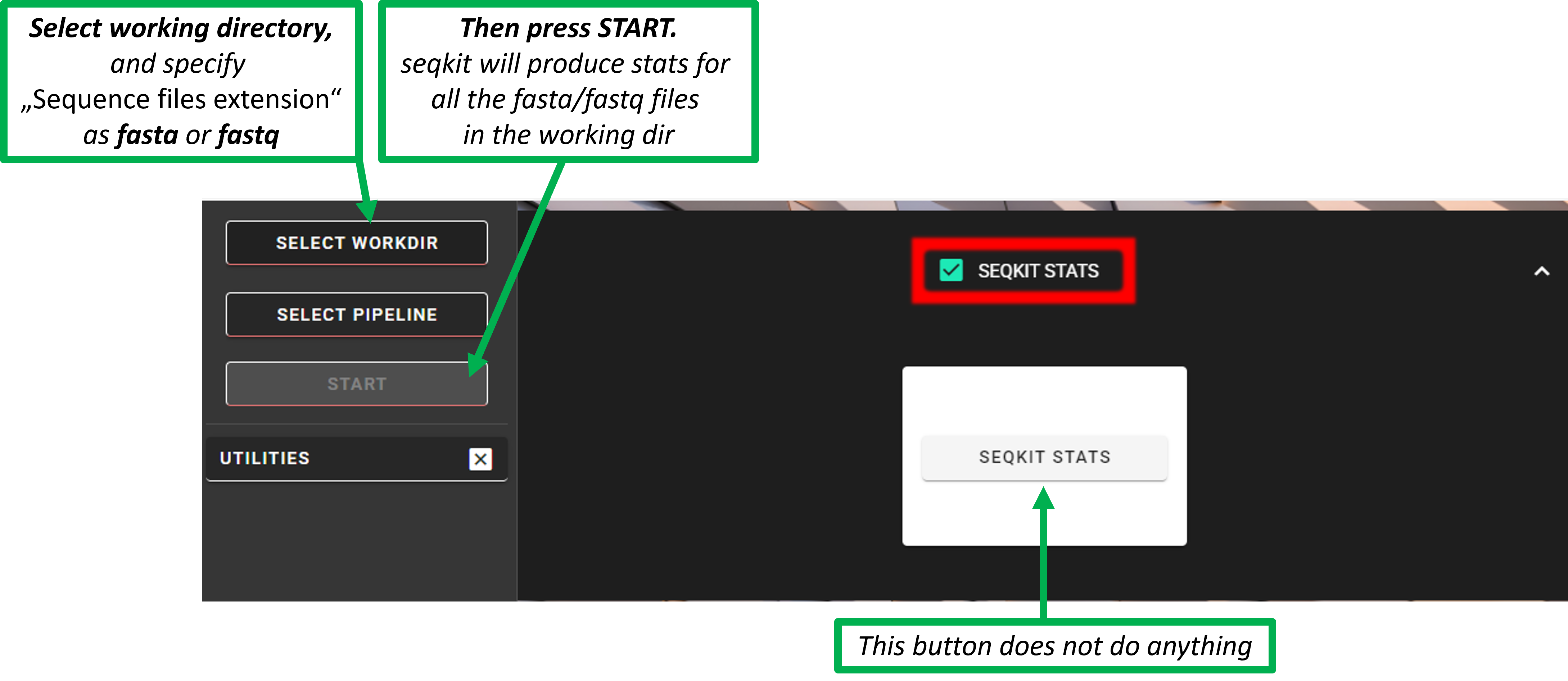
seqkit stats

Get sequence statistics with seqkit stats. Works with fasta(.gz)/fastq(.gz) files in the WORKING DIRECTORY.

Check the “SEQKIT STATS” box, press SELECT WORKDIR button to specify the working directory and Sequence files extension as fasta or fastq (Sequencing read types do not matter here, just click ‘Confirm’). Press START button –> seqkit will make stats for all fastq/fastq files in the working directory.

Output is the tab-delimited text file seqkit_stats.$fileFormat.txt with the following content:

Statistic	Description
file	Input file name
format	File format (FASTA/FASTQ)
type	Sequence type (DNA/RNA)
num_seqs	Number of sequences
sum_len	Total sequence length
min_len	Minimum sequence length
avg_len	Average sequence length
max_len	Maximum sequence length

Add sequences to table

This tool takes a feature table (abundance matrix: features as rows, samples as columns) and a feature FASTA whose sequence IDs match the feature identifiers in the table. It joins the corresponding sequences into the table as an extra column named ``Sequence``, inserted as the second column (after the feature ID column).

In PipeCraft2, steps such as ASV TO OTU expect the table to carry also sequences. If your table was exported without a Sequence column, run this tool before running ASV TO OTU.

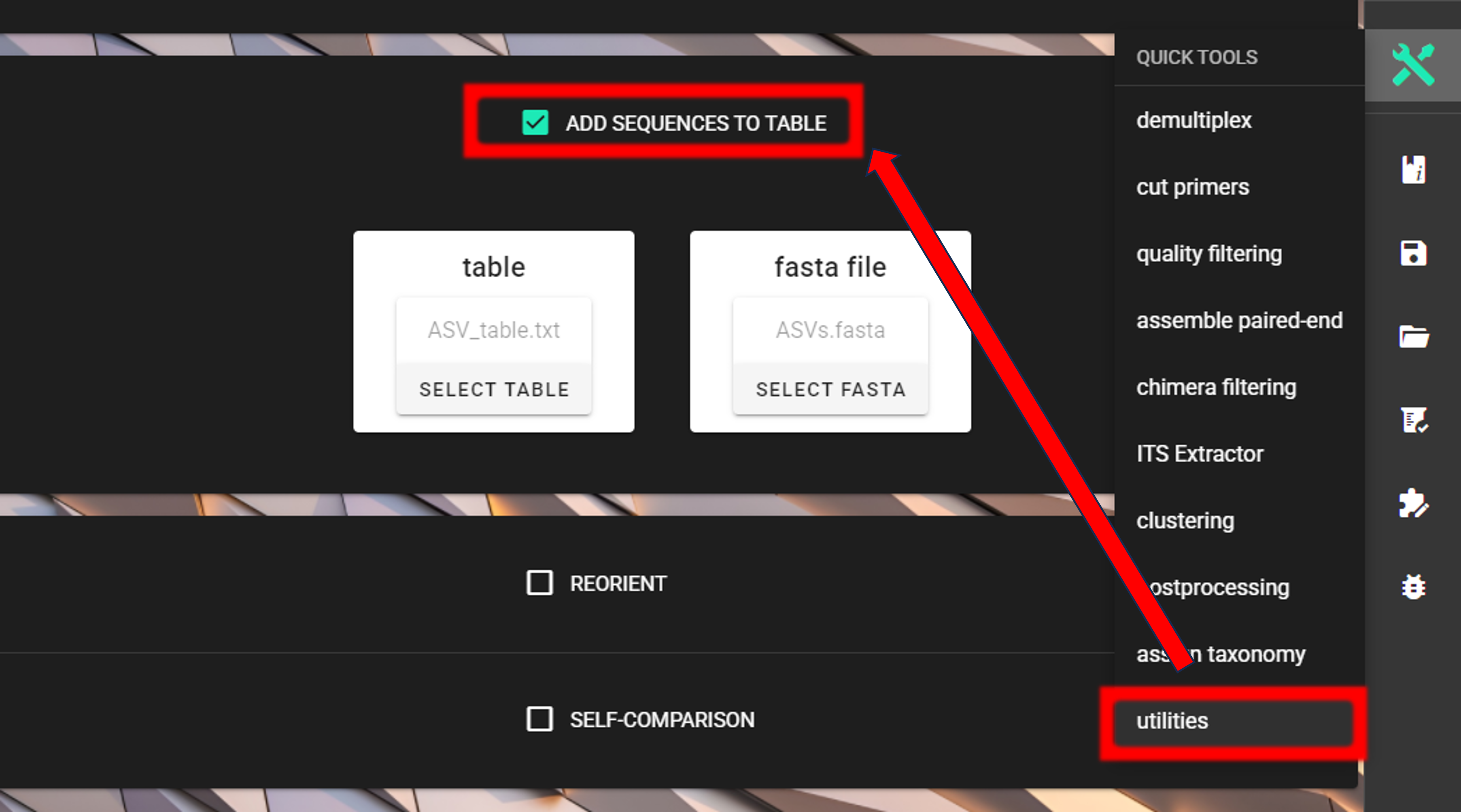
Output file, *_wSeqs.txt is in the same directory as specified with SELECT WORKDIR button.

Self-comparison

Run self-comparison of sequences in a fasta file to find identical or similar sequences within the same file. There are two methods implemented: BLAST and vsearch. This tool is useful for identifying duplicate, near-duplicate, or highly similar sequences within your dataset.

Note

To START, specify working directory under SELECT WORKDIR (will be the output directory), but the sequence files extension and read type (single-end or paired-end) do not matter here (just click ‘Confirm’).

Setting	Description
method	Choose between ‘vsearch’ or ‘blast’ for sequence comparison
fasta_file	Select input fasta file for self-comparison analysis
identity_threshold	Minimum sequence identity percentage to report matches (default: 60%)
coverage_threshold	Minimum sequence coverage percentage to report matches (default: 60%)
strand	both or plus

Outputs

Output is a tab-delimited text file in self_comparison_out directory.

vsearch output:

Column	Description
query	Query sequence identifier
target	Target sequence identifier
id	Sequence identity percentage
alnlen	Alignment length
qcov	Query coverage percentage
tcov	Target coverage percentage
ql	Query sequence length
tl	Target sequence length
ids	Number of identical positions
mism	Number of mismatches
gaps	Number of gap openings
qilo	Query alignment start position
qihi	Query alignment end position
qstrand	Query strand orientation (+/-)
tstrand	Target strand orientation (+/-)

BLAST output:

Column	Description
qseqid	Query sequence identifier
sseqid	Subject sequence identifier
pident	Percentage of identical matches
length	Alignment length
mismatch	Number of mismatches
gapopen	Number of gap openings
qstart	Query alignment start position
qend	Query alignment end position
sstart	Subject alignment start position
send	Subject alignment end position
evalue	Expect value
bitscore	Bit score
qlen	Query sequence length
slen	Subject sequence length
qcovs	Query coverage per subject
qcovhsp	Query coverage per high-scoring pair
sstrand	Subject strand orientation

reorient

Sequences are often (if not always) in both, 5’-3’ and 3’-5’, orientations in the raw sequencing data sets. If the data still contains PCR primers that were used to generate amplicons, then by specifying these PCR primers, this panel will perform sequence reorientation of all sequences.

Generally, this step is not needed when following vsearch OTUs or UNOISE ASVs pipeline, because both strands of the sequences can be compared prior forming OTUs (strand=both). This is automatically handled also in NextITS pipeline. In the DADA2 ASVs pipeline, if working with mixed orientation data (seqs in 5’-3’ and 3’-5’ orientations), then select PAIRED-END MIXED mode to account for mixed orientation data.

Process description: for reorienting, first the forward primer will be searched (using fqgrep) and if detected then the read is considered as forward complementary (5’-3’). Then the reverse primer will be searched (using fqgrep) from the same input data and if detected, then the read is considered to be in reverse complementary orientation (3’-5’). Latter reads will be transformed to 5’-3’ orientation and merged with other 5’-3’ reads. Note that for paired-end data, R1 files will be reoriented to 5’-3’ but R2 reads will be reoriented to 3’-5’ in order to merge paired-end reads.

At least one of the PCR primers must be found in the sequence. For example, read will be recorded if forward primer was found even though reverse primer was not found (and vice versa). Sequence is discarded if none of the PCR primers are found.

Sequences that contain multiple forward or reverse primers (multi-primer artefacts) are discarded as it is highly likely that these are chimeric sequences. Reorienting sequences will not remove primer strings from the sequences.

Note

For single-end data, sequences will be reoriented also during the ‘cut primers’ process (see below); therefore this step may be skipped when working with single-end data (such as data from PacBio machines OR already assembled paired-end data).

Supported file formats for paired-end input data are only fastq, but also fasta for single-end data. Outputs are fastq/fasta files in reoriented_out directory. Primers are not truncated from the sequences; this can be done using CUT PRIMER panel

Setting	Tooltip
`mismatches`	allowed mismatches in the primer search
`forward_primers`	specify forward primer (5’-3’); IUPAC codes allowed; add up to 13 primers
`reverse_primers`	specify reverse primer (3’-5’); IUPAC codes allowed; add up to 13 primers

Expert-mode (PipeCraft2 console)

Bioinformatic tools used by PipeCraft2 are stored on Dockerhub as Docker images. These images can be used to launch any tool with the Docker CLI to utilize the compiled tools. Especially useful in Windows OS, where majority of implemented modules are not compatible.

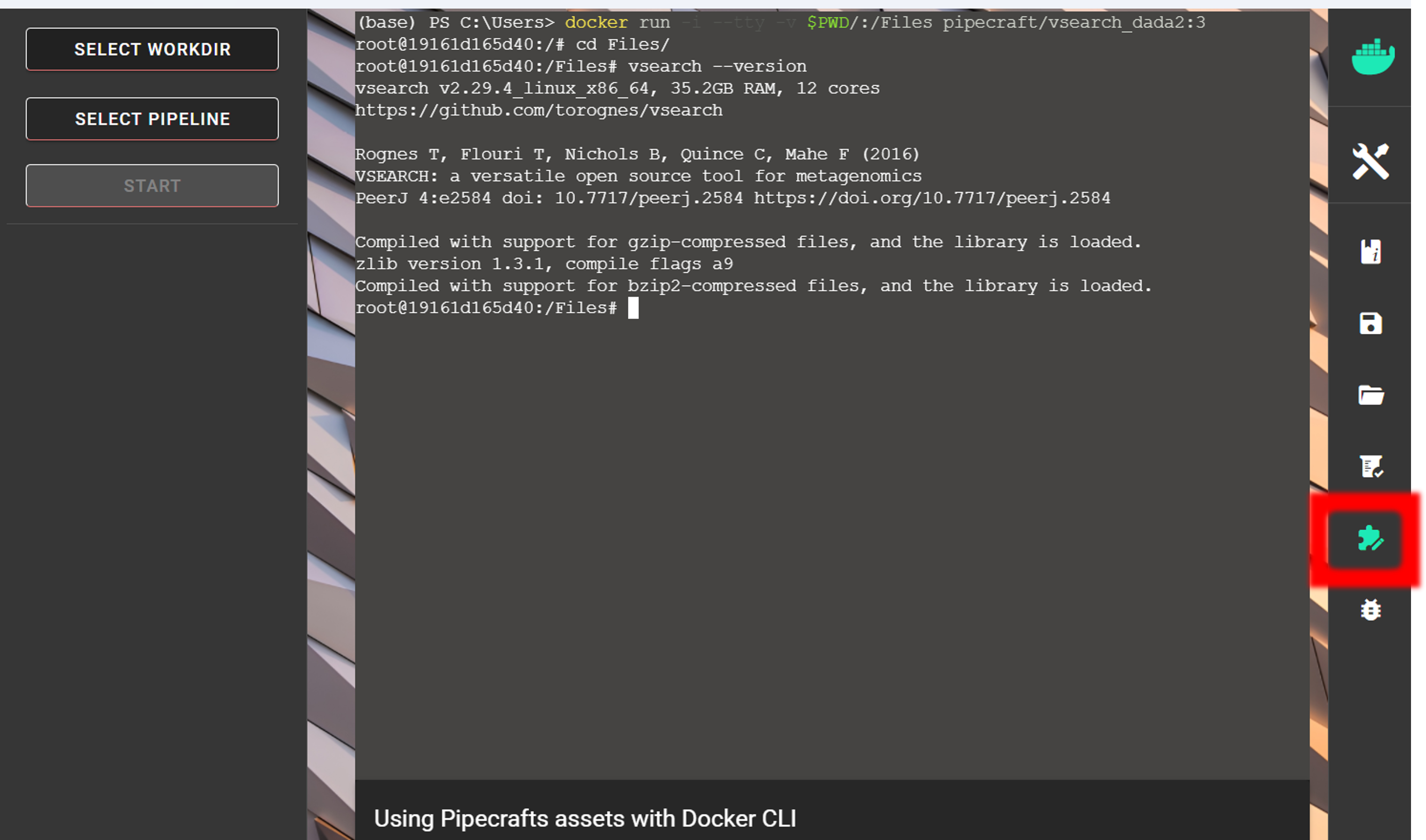
See list of docker images with implemented software here

Show a list of all images in your system (using e.g. Expert-mode):

docker images

Download an image if required (from Dockerhub):

docker pull pipecraft/IMAGE:TAG

docker pull pipecraft/vsearch:2.18

Delete an image

docker rmi IMAGE

docker rmi pipecraft/vsearch:2.18

Run docker container in your working directory to access the files. Outputs will be generated into the specified working directory. Specify the working directory under the -v flag:

docker run -i --tty -v users/Tom/myFiles/:/Files pipecraft/vsearch:2.18

Once inside the container, move to /Files directory, which represents your working directory in the container; and run analyses

cd Files
vsearch --help
vsearch *--whateversettings*

Exit from the container:

exit