DADA2 ASVs pipeline, 16S 
This example data analyses follows DADA2 ASVs workflow as implemented in PipeCraft2’s pre-compiled pipelines panel.
Starting point
This example dataset consists of 16S rRNA gene V4 amplicon sequences:
paired-end Illumina MiSeq data;
demultiplexed set (per-sample fastq files);
indexes and primers have already been removed;
sequences in this set are 5’-3’ (fwd) oriented.
when working with your own data …
… then please check that the paired-end data file names contain R1 and R2 strings (not just _1 and _2), so that PipeCraft can correctly identify the paired-end reads.
At least 2 samples (2x R1 + 2x R2 files) are required for this workflow! Otherwise ERROR in the denoising step:

SELECT PIPELINE –> DADA" ASVs.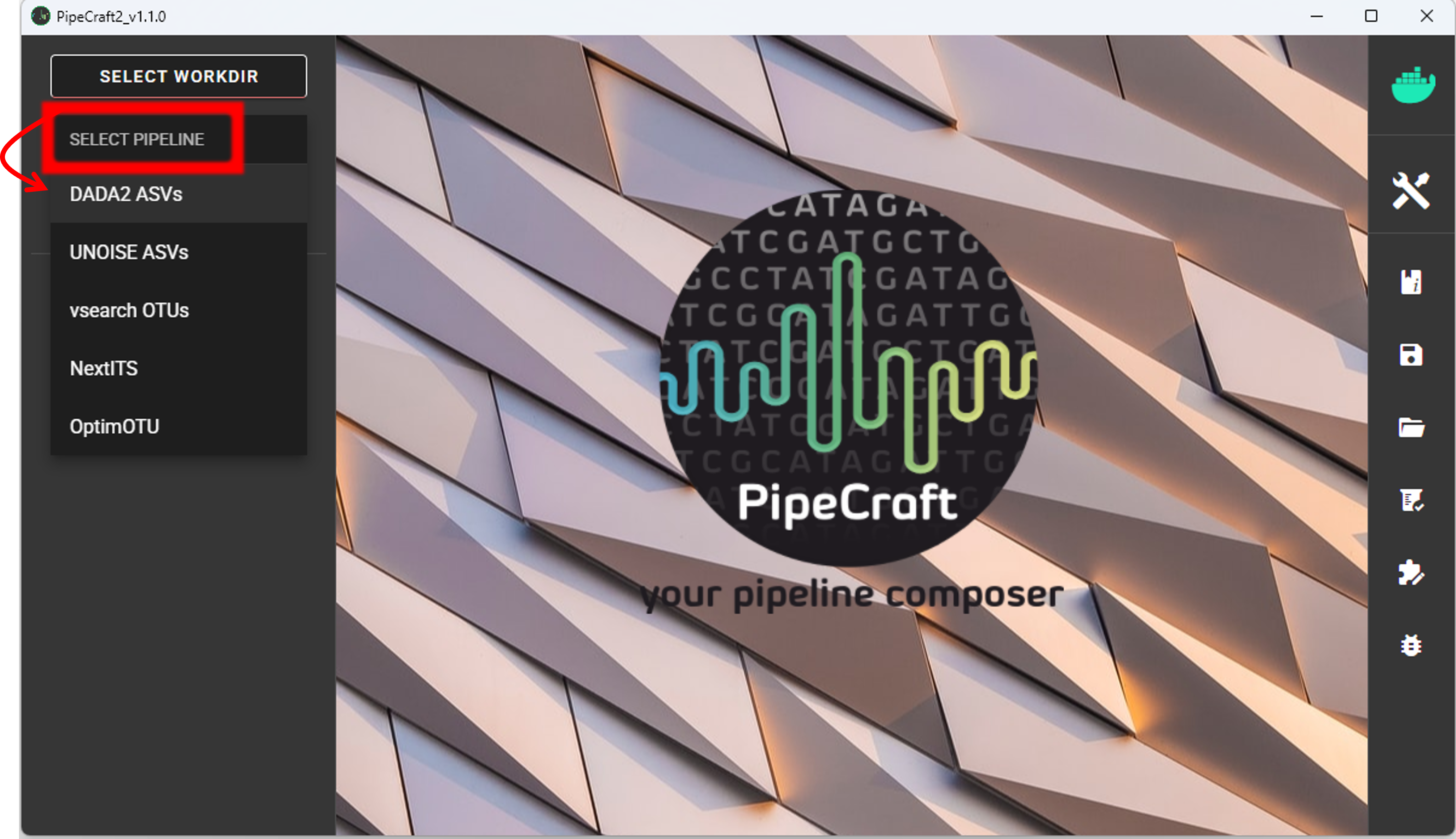
SELECT WORKDIRsequence files extension as *.fastq;sequencing read types as paired-end.MiSeq_SOP (note the in Windows, the directory files are not displayed).Workflow mode
Because we are working with sequences that are 5’-3’ oriented, we are selecting hte PAIRED-END FORWARD mode of the pipeline.

if sequences are in mixed orientation
If some sequences in your library are in 5’-3’ and some as 3’-5’ orientation, then with the ‘PAIRED-END FORWARD’ mode exactly the same ASV may be reported twice, where one ASV is just the reverse complementary of another. To avoid that, select PAIRED-END MIXED mode. Sequences have mixed orientation in libraries where sequenceing adapters have been ligated, rather than attached to amplicons during PCR.
Specifying primers (for CUT PRIMERS) is mandatory for the PAIRED-END MIXED mode. Based on the priemr sequences, the library will be split into two: 1) fwd oriented sequences, and 2) rev oriented sequences. Both batches are processed independently to produce ASVs, after which the rev oriented batch ASVs are reverse complemented and merged with the fwd oriented ASVs. Identical ASVs are merged to form a final data set. This is a reccomended workflow for accurate denoising compared with first reorienting all sequences to 5’-3’, and then performing a standard ‘PAIRED-END FORWARD’ workflow.
Cut primers
The example dataset has primers already clipped, so here we are skipping this process.
when working with your own data …
… and you need to clip primers, then check the box for CUT PRIMERS and specify the PCR primers. You may specify add up to 13 primer pairs. Check cut primers page.
Quality filtering
Before adjusting quality filtering settings, let’s have a look on the quality profile of our example data set.
Below quality profile plot was generated using QualityCheck panel (see here).

In this case, all R1 files are represented with green lines, indicating good average quality per file (i.e., sample). However, all R2 files are either yellow or red, indicating a drop in quality scores. Lower qualities of R2 reads are characteristic for Illumina sequencing data, and is not too alarming. DADA2 algoritm is robust to lower quality sequences, but removing the low quality read parts will improve the DADA2 sensitivity to rare sequence variants; so, let’s do some quality filtering.
Click on QUALITY FILTERING to expand the panel

Based on the quality scores distribution plot above, we will trim reads to specified length to remove low quality ends.
Set truncLen to 240 for trimming R1 reads and truncLen R2 to 160 to trim R2 reads.
Latter positions represent the approximate positions where sequence quality drops notably.
Alternatively, you may use trimLeft and trimRight options to remove bases from the start and end of the reads, respectively.
See also remove low-quality ends/starts of reads section.
when working with your own data …
… be sure to consider the amplicon length before applying truncLen options,
so that R1 and R2 reads would still overlap for the MERGE PAIRS process.
Non-overlapping paired-end reads will be discarded.
Here, we can leave other settings as DEFAULT.
Output directory |
|
|---|---|
*.fastq |
quality filtered sequences per sample in FASTQ format |
*.rds |
R objects for the following DADA2 workflow processes |
seq_count_summary.csv |
summary of sequence counts per sample |
Denoise and merge pairs
This step performs desiosing (as implemented in DADA2), which first forms ASVs per R1 and R2 files. Then during merging/assembling process the paired ASV mates are assembled to output full amplicon length ASV.

Here, we are working with Illumina MiSeq data, so let’s make sure that the errorEstFun setting is loessErrfun. For PacBio data use PacBioErrfun.
We can leave all settings as DEFAULT.
Output directory |
|
|---|---|
*.fasta |
denoised and assembled ASVs per sample in FASTA format |
*.rds |
R objects for the following DADA2 workflow processes |
Error_rates_R*.pdf |
plots for estimated R1/R2 error rates |
seq_count_summary.csv |
summary of sequence counts per sample |
Chimera filtering
This step performs chimera filtering according to DADA2 removeBimeraDenovo function. During this step, the ASV table is also generated.
Important
make sure that primers have been removed from your amplicons; otherwise many false-positive chimeras may be filtered out from your dataset.
Here, we filter chimeras using the consensus method.
Output directory |
|
|---|---|
*.fasta |
chimera filtered ASVs per sample |
seq_count_summary.csv |
summary of sequence counts per sample |
‘chimeras’ dir |
ASVs per sample identified as chimeras |
Output directory |
|
|---|---|
ASVs_table.txt |
denoised and chimera filtered ASV-by-sample table |
ASVs.fasta |
corresponding FASTA formated ASV Sequences |
ASVs per sample identified as chimeras |
rds formatted denoised and chimera filtered ASV table |
Curate ASV table
This process first removes putative tag jumps and then collapses the ASVs that are identical up to shifts or length variation, i.e. ASVs that have no internal mismatches (PipeCraft2 uses vsearch usearch_global –id 1 for that); and finally filters out ASVs that are shorter/longer than specified length (in base pairs).

Here, we are enabling this process by checking the box for CURATE ASV TABLE in the DADA2 ASV workflow panel.
The f_value and p_value settings are used to filter out putative tag jumps (using UNCROSS2 algorithm).
Generally, we recommend to use p_value of 1 (default), and f_value of 0.03 when using combinational indexing strategy;
f_value of 0.05 when using single-indexes, and f_value of 0.01 when using unique dual-indexes.
The expected amplicon length (without primers) in our example dataset in ~253 bp.
Assuming that shorter sequences are non-target sequences,
we use 240 in the min length setting. This will discard ASVs that are less than 240 bp.
Here, max length can be set to 0 (default), meaning no filtering by maximum sequence length.
We are also setting the collapseNoMismatch to TRUE, to collapse identical ASVs.
This is basically equivalent to 100% clustering by ignoring the end gaps.
Output directory |
|
|---|---|
ASVs_table_TagJumpFilt.txt |
only tag-jump filtered ASV-by-sample table |
ASVs.fasta |
corresponding ASV Sequences with ASVs_table_TagJumpFilt.txt table |
ASVs_collapsed.fasta
|
tag-jump filtered and collapsed and size filtered
ASV Sequences. Present only if some ASVs were collapsed.
|
ASVs_table_collapsed.txt
|
corresponding ASV-by-sample table.
Present only if some ASVs were collapsed.
|
TagJump_stats.txt |
summary of tag-jump filtering results |
If there is nothing to collapse or filter out based on the length
then there are no corresponding files in the ASVs_out.dada2/curated directory, and only
ASVs_table_TagJumpFilt.txt and ASVs.fasta files will be generated
(even when there is nothing to tag-jump filter - in which case ASVs_table_TagJumpFilt.txt is the same
ASVs_table.txt in the ASVs_out.dada2 directory).
Note
The pre-compiled pipeline ends here. Outputs 16S ASVs can be further clustered into OTUs.
Save workflow
Once we have decided about the settings in our workflow, we can save the configuration file by pressing save workflow button on the right-ribbon

If you forget the save, then no worries, a pipecraft2_last_run_configuration.json file will be generated
for you upon starting the workflow.
As the file name says, it is the workflow configuration file for your last PipeCraft run in this working directory.
If the file name (pipecraft2_last_run_configuration.json) is not changed, then the file is overwritten with the new configuration
if running a new job in the same working directory.
This JSON file can be loaded into PipeCraft2 to automatically configure your next runs exactly the same way.
Note
‘Assign taxonomy’ is not the part of the full per-defined pipeline. This step can be selected and run via QuickTools panel. See below.
Start the workflow
Press START on the left ribbon to start the analyses.
when running the module for the first time …
… a docker image will be first pulled to start the process.
For example: 
When you need to STOP the workflow, press STOP button 
When the workflow has completed …
… a message window will be displayed.

Assign taxonomy
Assign taxonomy is not the part of the full per-defined pipeline, but can be run as a separate step in QuickTools.
Double-check the selected working directory (the outputs will be written there) by holding
the mouse cursor over the SELECT WORKDIR button [re-select if needed].
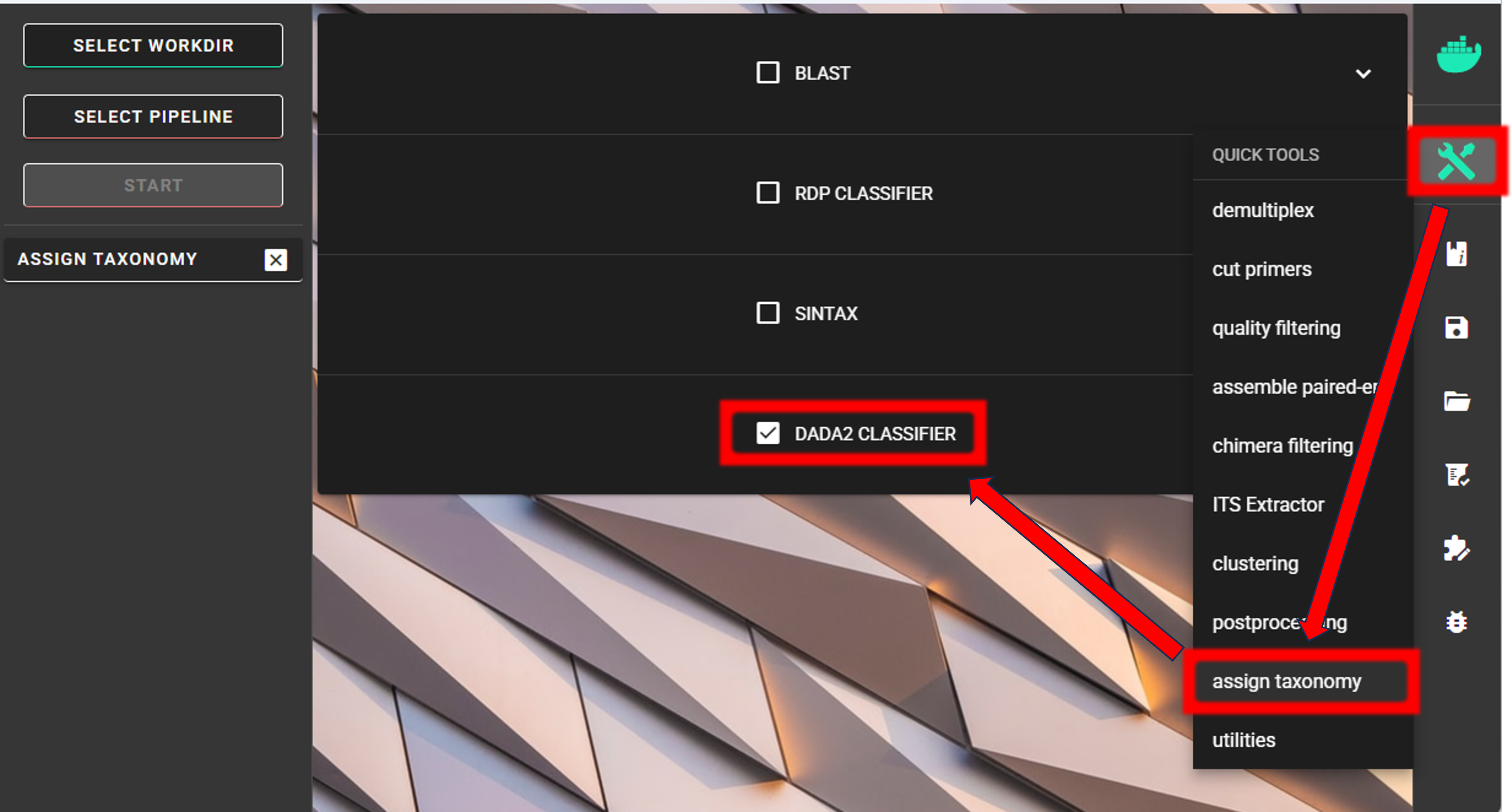
Here, we are using the DADA2 classifier, the assignTaxonomy function, which itself implements the RDP Naive Bayesian Classifier algorithm. See other assign taxonomy options here.
We need to specify the location of the reference DATABASE for the taxonomic classification of our ASVs. Click on the header of dada2_database setting,
which directs you to the DADA2-formatted reference databases web page.
Here, we are using silva_nr99_v138.2_toSpecies_trainset.fa.gz.
See other databases available for taxonomy annotation here.

Specify the location of your downloaded database and also the fasta file with ASVs (fasta file) to be classified.
Herein, we use ASVs.fasta file in the ASVs_out.dada2/curated directory (since we applied also CURATE ASV TABLE process).
We can use the default minBoot (minimum bootstrap; ranging from 0-100; ~assignment confidence) value of 80.
This means that taxonomic ranks with at least bootstrap value of 80 will get classification (unclassified for <80).
tryRC may be OFF, since we expact that all of our ASVs are in 5’-3’ orientation.
Press “START” to start the taxonomy assignment process.
Output directory |
|
|---|---|
taxonomy.csv |
classifier results with bootstrap values |
Examine the outputs
Several process-specific output folders are generated ![]()
|
quality filtered paired-end fastq files per sample |
|
denoised and assembled fasta files per sample |
|
chimera filtered fasta files per sample |
|
ASVs table, and ASV sequences files |
|
curated ASVs table, and ASV sequences files |
|
ASVs taxonomy table (taxonomy.csv) |
Each folder (except ASVs_out.dada2 and taxonomy_out.dada2) contain
summary of the sequence counts (seq_count_summary.csv).
Examine those to track the read counts throughout the pipeline.
For example, from the seq_count_summary.csv file in qualFiltered_out we see that on average ~91% of the sequences survived the quality filtering step.
input |
qualFiltered |
|
F3D0_S188_L001 |
7793 |
7113 |
F3D1_S189_L001 |
5869 |
5299 |
F3D141_S207_L001 |
5958 |
5463 |
F3D142_S208_L001 |
3183 |
2914 |
F3D143_S209_L001 |
3178 |
2941 |
… |
Here, we applied also “CURATE ASV TABLE” process.
Therefore, our final outputs of the pipeline are in the ASVs_out.dada2/curated directory.
ASVs_out.dada2/curated directory contains ASVs_table_TagJumpFilt.txt file.
This represents the ASV table after the tag-jump filtering,
where the 1st column represents ASV identifiers (sha1 encoded),
2nd column is the sequence of an ASV,
and all the following columns represent number of sequences in the corresponding samples
(sample name is taken from the file name). This is tab delimited text file.
ASVs_table_TagJumpFilt.txt; first 4 samples and 4 ASVs:
OTU |
Sequence |
F3D0_S188_L001 |
F3D1_S189_L001 |
F3D141_S207_L001 |
7c6864ace… |
TACGGAG… |
579 |
405 |
444 |
1e3c68bda… |
TACGGAG… |
345 |
353 |
362 |
4ee096262… |
TACGGAG.. |
449 |
231 |
345 |
1cf2c5b8e… |
TACGGAG… |
430 |
69 |
164 |
Note: even though the ASVs column header is “OTU”, it represents ASVs as we preformed an ASVs workflow!
The ASV + Sequences info are also represented in the fasta file (ASVs.fasta) in the ASVs_out.dada2 directory.
did ‘CURATE ASV TABLE’ have any effect?
In this example, we applied also collapseNoMismatch and min length filtering.
If we examine the README.txt file in the ASVs_out.dada2/curated directory,
then we see a note “Output has the same number of Features (ASVs/OTUs) as input”,
which means that no ASVs were filtered out based on the collapseNoMismatch and min length filters.
Thus, ASVs_table.txt and ASVs.fasta files in the ASVs_out.dada2 directory
contain the same number of ASVs.
However, we applied also tag-jump filtering process (via f_value and p_value settings).
When checking the TagJump_stats.txt file in the ASVs_out.dada2/curated directory,
we see that based on our settings, 9 tag-jump events were detected which involved 78 reads.
That is, there were 9 potential cases where an ASV may have been “leaked” from one sample to another.
The number of ASVs are the same in ASVs_out.dada2/curated/ASVs_table_TagJumpFilt.txt and ASVs_out.dada2/ASVs_table.txt files,
but ASVs_table_TagJumpFilt.txt file has 78 less reads than “ASVs_table.txt” file as those were removed as putative tag-jumps.
So, for further processes, we use ASVs_table_TagJumpFilt.txt file,
and ASVs.fasta file in the ASVs_out.dada2/curated directory.
Result from the taxonomy annotation process - taxonomy table (taxonomy.csv) - is located at the taxonomy_out.dada2 directory.
Taxonomy results for the first 5 ASVs
ASV |
Sequence |
Kingdom |
Phylum |
Class |
Order |
Family |
Genus |
Species |
Kingdom |
Phylum |
Class |
Order |
Family |
Genus |
Species |
7c6864ace… |
TACGGAG… |
Bacteria |
Bacteroidota |
Bacteroidia |
Bacteroidales |
Muribaculaceae |
NA |
NA |
100 |
100 |
100 |
100 |
100 |
100 |
100 |
1e3c68bda… |
TACGGAG… |
Bacteria |
Bacteroidota |
Bacteroidia |
Bacteroidales |
Muribaculaceae |
NA |
NA |
100 |
100 |
100 |
100 |
100 |
100 |
100 |
4ee096262… |
TACGGAG.. |
Bacteria |
Bacteroidota |
Bacteroidia |
Bacteroidales |
Muribaculaceae |
NA |
NA |
100 |
100 |
100 |
100 |
100 |
98 |
98 |
1cf2c5b8e… |
TACGGAG… |
Bacteria |
Bacteroidota |
Bacteroidia |
Bacteroidales |
Muribaculaceae |
NA |
NA |
100 |
100 |
100 |
100 |
100 |
100 |
82 |
57bde09f1… |
TACGGAG… |
Bacteria |
Bacteroidota |
Bacteroidia |
Bacteroidales |
Bacteroidaceae |
Bacteroides |
caecimuris |
100 |
100 |
100 |
100 |
100 |
100 |
100 |
“NA” denotes that the sequence may not have enough resolution to confidently (herein we used minimum bootstrap of 80) place that ASV within a specific taxonomic rank or the database lack of reference sequences for more accurate classification. Last columns with integers (for ‘Kingdom’ to ‘Species’) represent bootstrap values for the correspoinding taxonomic unit.
Check for the non-target hits
It is often the case that universal metabarcoding primers amplify also non-target DNA regions and/or non-target taxa. Working with this example dataset, we are interesed only in Bacteria, thus we should get rid of the off-target noise before proceeding with relevant statistical analyses.
When we carefully examine the results, the taxonomy table, then we can see that 3 ASVs are classified as Chloroplast (‘Order’ column) and 1 ASVs as Mitochondria (‘Family’ column).
ASV |
Sequence |
Kingdom |
Phylum |
Class |
Order |
Family |
Genus |
Species |
Kingdom |
Phylum |
Class |
Order |
Family |
Genus |
Species |
5c25197ab1565ef226075d05cff73a9cee0e3a2f |
GACAG… |
Bacteria |
Cyanobacteria |
Cyanobacteriia |
Chloroplast |
NA |
NA |
NA |
100 |
100 |
100 |
100 |
100 |
100 |
100 |
1c167d19cce4b4113c12dde61306132efed8dc20 |
GACAG… |
Bacteria |
Cyanobacteria |
Cyanobacteriia |
Chloroplast |
NA |
NA |
NA |
100 |
100 |
100 |
100 |
100 |
100 |
100 |
2f24601af9870b6120292e9f8a8280362d8ff0e0 |
GACAG… |
Bacteria |
Cyanobacteria |
Cyanobacteriia |
Chloroplast |
NA |
NA |
NA |
100 |
100 |
100 |
100 |
100 |
100 |
100 |
e488265f509c969b5b2f63e7345c13417ed66035 |
GACGG… |
Bacteria |
Proteobacteria |
Alphaproteobacteria |
Rickettsiales |
Mitochondria |
NA |
NA |
100 |
100 |
100 |
100 |
100 |
100 |
100 |
The PCR primers used to generate the amplicon library, 515F and 806R, match very well with regions in the chloroplast and mitochondria genomes; and amplyfy also ~250 bp fragments which are nicely sequenced alongside with the bacterial 16S fragments. Chloroplast sequences are similar to ones in Cyanobacteria, and mitochondria sequences to ones in Rickettsiales (because of evolutionary history of these organelles), therewere we see these sequences in Phylum Cyanobacteria and Order Rickettsiales in the SILVA database, respectivelly. However, when flagged as “Chloroplast” or “Mitochondria”, then those sequences most likely originate from the corresponding organelle genomes not from the bacterial 16S rRNA.
It is common obtain these kind of off-target sequences from environmental DNA samples (such as soil, water) since the DNA pool likely contains also plant or algal DNA. Chloroplast|mitochondria are not present in bacteria (or Archaea), therefore ASVs with assignments to Chloroplast and/or Mitochondria can be considered off-target ASVs and should be removed.
Below, you can find a R script to clean your taxonomy table, ASV table and ASVs fasta file from the off-target taxa and from ‘Chloroplast’ and ‘Mitochondria’ sequences.
 1 #!/usr/bin/env Rscript
 2 # This is R script.
 3
 4 ### Filter taxonomy table, ASV table and ASVs fasta file to exclude non-target ASVs
 5
 6 # specify input tables and fasta file
 7 taxonomy_table = "taxonomy.csv"          # csv file
 8 ASV_table = "ASVs_table_TagJumpFilt.txt" # tab-delimited file
 9 ASV_fasta = "ASVs.fasta"                 # FASTA file
10 #----------------------------------------------------------#
11
12 library(dplyr)
13 library(readr)
14
15 # load the taxonomy and ASV table
16 taxonomy = read.csv(taxonomy_table, header = TRUE)
17 ASV_table = read_tsv(ASV_table)
18
19 # make sure that the first column header is "ASV"
20 if (colnames(taxonomy)[1] != "ASV") {
21   colnames(taxonomy)[1] = "ASV"
22 }
23 if (colnames(ASV_table)[1] != "ASV") {
24   colnames(ASV_table)[1] = "ASV"
25 }
26
27 # double-check that all Kingdom level classifications are "Bacteria" or "Archaea"
28 # change tax level and tax_group as needed
29 tax_level = "Kingdom"
30 tax_group = "Bacteria|Archaea"
31 target_taxonomy = taxonomy %>%
32   filter(grepl(tax_group, .[[tax_level]]))
33
34 # summary
35 if (nrow(taxonomy) - nrow(target_taxonomy) == 0) {
36   cat("\n All",tax_level, "level classifications are Bacteria|Archaea \n\n")
37 } else {
38   cat("\n", nrow(taxonomy) - nrow(target_taxonomy), "non", tax_group, "ASVs removed\n\n")
39 }
40
41 ## filter "Chloroplast|Mitochondria"
42 # a function to check for the presence of "Chloroplast" or "Mitochondria"
43 # in any column in taxonomy
44 chloroplast_or_mitochondria = function(row) {
45   any(grepl("Chloroplast|Mitochondria", row))
46 }
47
48 # filter out rows that contain Chloroplast or Mitochondria
49 filtered_taxonomy = target_taxonomy %>%
50   filter(!apply(., 1, chloroplast_or_mitochondria))
51
52 # summary
53 if (nrow(target_taxonomy) - nrow(filtered_taxonomy) == 0) {
54   cat("\n None of the target_taxonomy ASVs were classified as Chloroplast|Mitochondria \n\n")
55 } else {
56   cat("\n Removed", nrow(target_taxonomy) - nrow(filtered_taxonomy),
57                             "Chloroplast|Mitochondria ASVs.\n\n")
58 }
59
60 # write the filtered taxonomy table to a new file
61 write.csv(filtered_taxonomy, "filtered_taxonomy.csv", row.names = FALSE)
62
63
64 ### filter the ASV table ->
65 # get the list of good ASVs
66 good_ASVs = filtered_taxonomy$ASV
67
68 # Filter the ASV table to keep only "good ASVs"
69 filtered_ASV_table = ASV_table %>%
70   filter(ASV %in% good_ASVs)
71
72 # write the filtered ASV table to a new file
73 write.table(filtered_ASV_table, "taxFiltered_ASV_table.txt",
74             sep = "\t", quote = F, row.names = F)
75
76
77 ## filter the ASVs.fasta
78 library("seqinr")
79 # read the FASTA file
80 ASV_fasta = read.fasta(file = ASV_fasta,
81                       seqtype = "DNA")
82
83 # filter ASV_fasta to include only "good ASVs"
84 filtered_ASV_fasta = ASV_fasta[names(ASV_fasta) %in% good_ASVs]
85
86 # convert sequences to uppercase
87 filtered_ASV_fasta = lapply(filtered_ASV_fasta, toupper)
88
89 # write the filtered ASV fasta to a new file
90 write.fasta(sequences = filtered_ASV_fasta,
91             names = names(filtered_ASV_fasta),
92             nbchar = 999,
93             file.out = "taxFiltered_ASVs.fasta")
Final curated files
Now, final curated files are:
filtered_taxonomy.csvtaxFiltered_ASV_table.txttaxFiltered_ASVs.fasta
Proceed with any relevant statistical analyses using the curated files.