DADA2 ASVs pipeline, ITS2

This example data analyses follows vsearch OTUs workflow as implemented in PipeCraft2’s pre-compiled pipelines panel.

Download example data set here (15.1 Mb) and unzip it.

This is ITS2 Illumina MiSeq dataset.

For this example, we are using EUKARYOME database in the taxonomy annotation process (SINTAX). Download the SINTAX_EUK_ITS file from here and unzip it (note: use 7-Zip software for unzipping files in Windows).

---

Starting point

This example dataset consists of ITS2 rRNA gene amplicon sequences; targeting fungi:

• paired-end Illumina MiSeq data;

• demultiplexed set (per-sample fastq files);

• primers are not removed;

• sequences in this set are 5’-3’ oriented.

when working with your own data …

… then please check that the paired-end data file names contain R1 and R2 strings (not just _1 and _2), so that PipeCraft can correctly identify the paired-end reads.

Example:

sample1_R1.fastq.gz

sample1_R2.fastq.gz

At least 2 samples (2x R1 + 2x R2 files) are required for this workflow! Otherwise ERROR in the denoising step:

---

To select DADA2 pipeline, press

SELECT PIPELINE –> DADA" ASVs.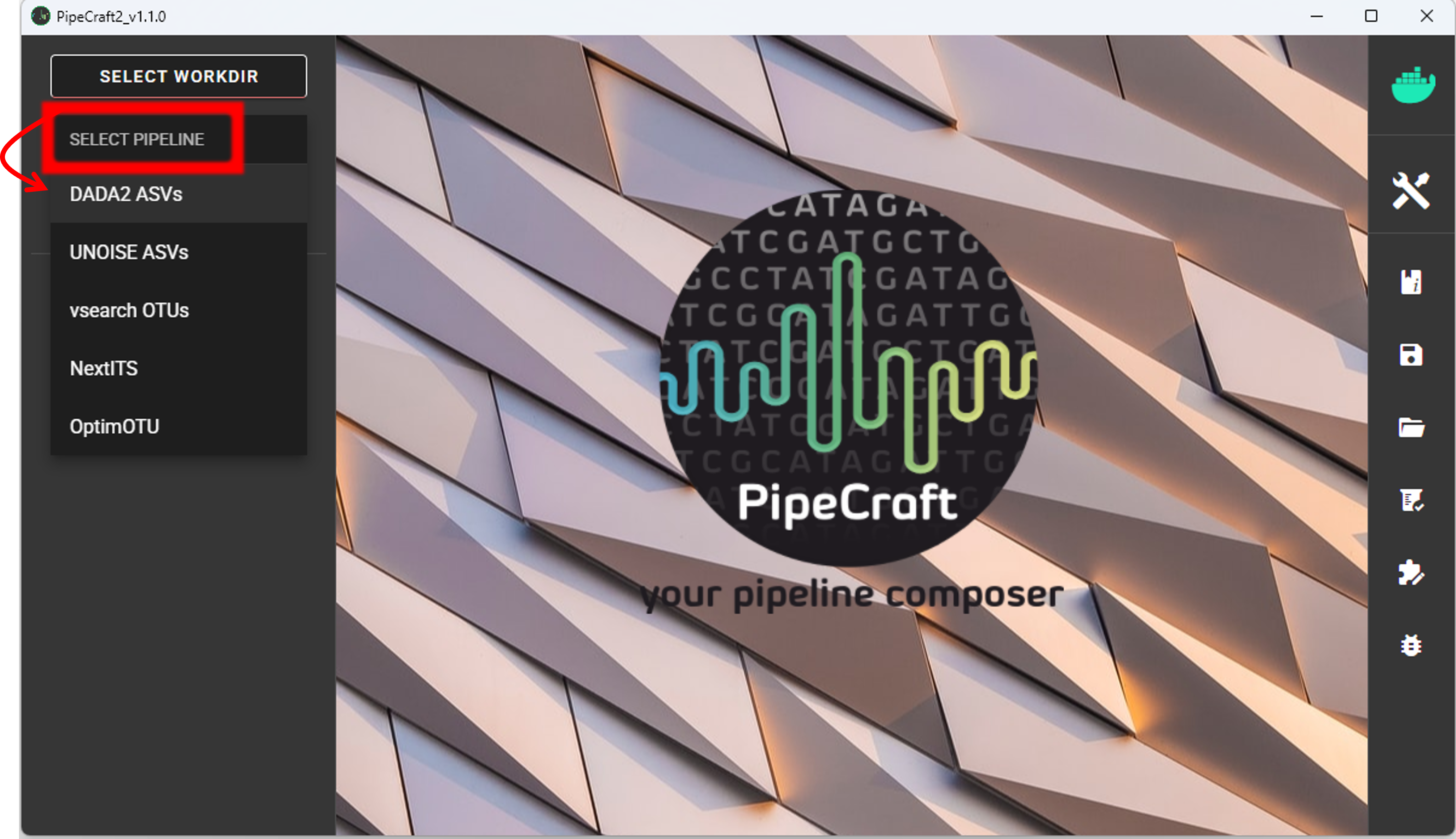

To select input data, press SELECT WORKDIR

and specify

sequence files extension as *.fastq.gz;

sequencing read types as paired-end.

---

Workflow mode

Because we are working with sequences that are 5’-3’ oriented, we are selecting hte PAIRED-END FORWARD mode of the pipeline.

if sequences are in mixed orientation

If some sequences in your library are in 5’-3’ and some as 3’-5’ orientation, then with the ‘PAIRED-END FORWARD’ mode exactly the same ASV may be reported twice, where one ASV is just the reverse complementary of another. To avoid that, select PAIRED-END MIXED mode. Sequences have mixed orientation in libraries where sequenceing adapters have been ligated, rather than attached to amplicons during PCR.

Specifying primers (for CUT PRIMERS) is mandatory for the PAIRED-END MIXED mode. Based on the priemr sequences, the library will be split into two: 1) fwd oriented sequences, and 2) rev oriented sequences. Both batches are processed independently to produce ASVs, after which the rev oriented batch ASVs are reverse complemented and merged with the fwd oriented ASVs. Identical ASVs are merged to form a final data set. This is a reccomended workflow for accurate denoising compared with first reorienting all sequences to 5’-3’, and then performing a standard ‘PAIRED-END FORWARD’ workflow.

---

Cut primers

The example dataset contains primer sequences. Generally, we need to remove these to proceed the analyses only with the variable metabarcode of interest. If there are some additional sequence fragments, from eg. sequencing adapters or poly-G tails, then clipping the primers will remove those fragments as well.

Tick the box for CUT PRIMERS and specify forward and reverse primers. For the example data, the forward primer is GTGARTCATCGAATCTTTG (fITS7) and reverse primer is TCCTCCGCTTATTGATATGC (ITS4).

Forward primer has 19 bp and reverse 20 bp - to keep a bit of flexibility in the primer search, we are requesting the min overlap of 18 bp and are allowing maximum of 2 mismatches . Note that too low min overlap may lead to random matches. Check other CUT PRIMER options here.

Note

You may specify add up to 13 primer pairs.

A consideration when working with ITS sequences and plan to use ITS Extractor

Since fITS7 and ITS4 primer binding sites are >50 bp from ITS2 region from the 5.8S side and >40 bp from the 28S side, we can clip the primers in order to safely use ITS Extractor to remove the flanking regions from ITS2 reads.

However, when the primer binding sites are very close to the ITS region (< 25 bp), then you may want to keep the primers for better detection of the 18S, 5.8S and 28S regions.

---

Quality filtering

Quality filtering removes sequences, which do not meet the specified quality threshold.

Click on QUALITY FILTERING to expand the panel

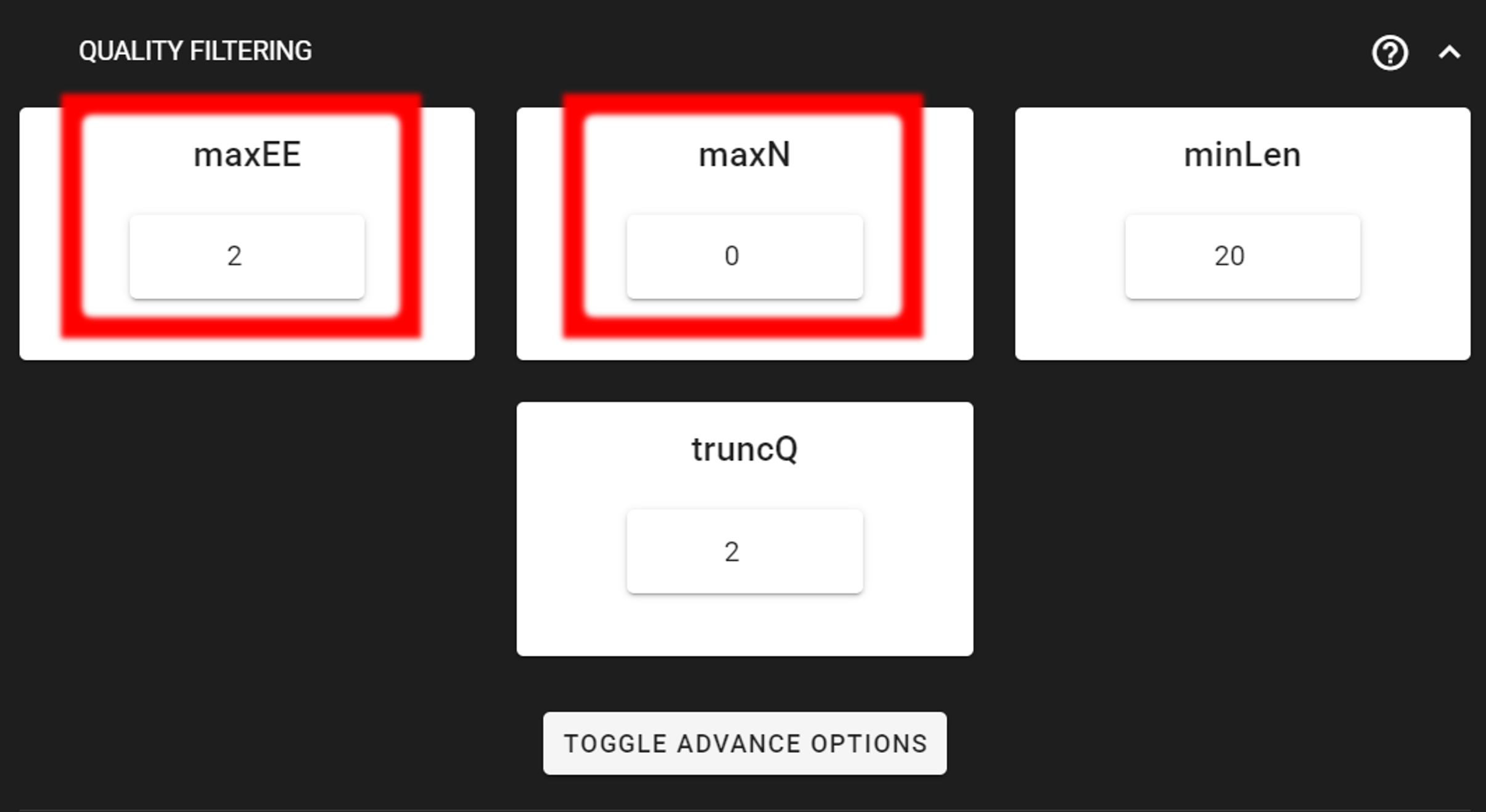
Here, we can leave the settings as DEFAULT by discarding sequences with maximum error rate of >2 and with ambiguous bases of >0. But based on your own data quality profile, you may need to adjust the settings. See also remove low-quality ends/starts of reads section.

Output directory qualFiltered_out
*.fq.gz	quality filtered sequences per sample in FASTQ format
*.rds	R objects for the following DADA2 workflow processes
seq_count_summary.csv	summary of sequence counts per sample

---

Denoise and merge pairs

This step performs desiosing (as implemented in DADA2), which first forms ASVs per R1 and R2 files. Then during merging/assembling process the paired ASV mates are assembled to output full amplicon length ASV.

Here, we are working with Illumina data, so let’s make sure that the errorEstFun setting is loessErrfun. We can leave all settings as DEFAULT.

Output directory denoised_assembled.dada2
*.fasta	denoised and assembled ASVs per sample in FASTA format
*.rds	R objects for the following DADA2 workflow processes
Error_rates_R*.pdf	plots for estimated R1/R2 error rates
seq_count_summary.csv	summary of sequence counts per sample

---

Chimera filtering

This step performs chimera filtering according to DADA2 removeBimeraDenovo function. During this step, the ASV table is also generated.

Important

make sure that primers have been removed from your amplicons; otherwise many false-positive chimeras may be filtered out from your dataset.

Here, we filter chimeras using the consensus method.

Output directory chimeraFiltered_out.dada2
*.fasta	chimera filtered ASVs per sample
seq_count_summary.csv	summary of sequence counts per sample
‘chimeras’ dir	ASVs per sample identified as chimeras

Output directory ASVs_out.dada2
ASVs_table.txt	denoised and chimera filtered ASV-by-sample table
ASVs.fasta	corresponding FASTA formated ASV Sequences
ASVs per sample identified as chimeras	rds formatted denoised and chimera filtered ASV table

---

Curate ASV table

This process first removes putative tag jumps and then collapses the ASVs that are identical up to shifts or length variation, i.e. ASVs that have no internal mismatches (PipeCraft2 uses vsearch usearch_global –id 1 for that); and finally filters out ASVs that are shorter/longer than specified length (in base pairs).

Here, we are enabling this process by checking the box for CURATE ASV TABLE in the DADA2 ASV workflow panel.

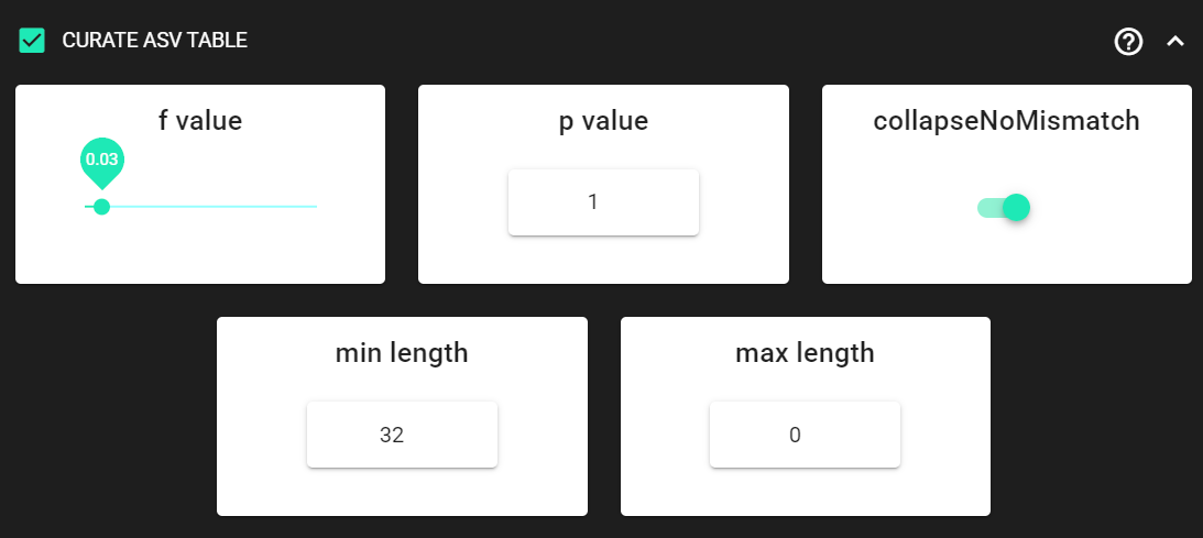
The f_value and p_value settings are used to filter out putative tag jumps (using UNCROSS2 algorithm). Generally, we recommend to use p_value of 1 (default), and f_value of 0.03 when using combinational indexing strategy; f_value of 0.05 when using single-indexes, and f_value of 0.01 when using unique dual-indexes.

We are setting the collapseNoMismatch to TRUE, to collapse identical ASVs. This is basically equivalent to 100% clustering by ignoring the end gaps.

Since the ITS2 amplicon length is highly variable, we are keeping min length and max length settings as default. max length is set to 0, meaning no filtering by maximum sequence length.

Output directory ASVs_out.dada2/curated
ASVs_table_TagJumpFilt.txt	only tag-jump filtered ASV-by-sample table
ASVs.fasta	corresponding ASV Sequences with ASVs_table_TagJumpFilt.txt table
ASVs_collapsed.fasta	tag-jump filtered and collapsed and size filtered ASV Sequences. Present only if some ASVs were collapsed.
ASVs_table_collapsed.txt	corresponding ASV-by-sample table. Present only if some ASVs were collapsed.
TagJump_stats.txt	summary of tag-jump filtering results

If there is nothing to collapse or filter out based on the length

then there are no corresponding files in the ASVs_out.dada2/curated directory, and only ASVs_table_TagJumpFilt.txt and ASVs.fasta files will be generated (even when there is nothing to tag-jump filter - in which case ASVs_table_TagJumpFilt.txt is the same ASVs_table.txt in the ASVs_out.dada2 directory).

Note

The pre-compiled pipeline ends here. Outputs ITS2 ASVs can be further filtered to remove flanking gene fragments from ITS2 sequences (via ITS Extractor), and optionally ASVs can be clustered into OTUs. See below.

---

Save workflow

Once we have decided about the settings in our workflow, we can save the configuration file by pressing save workflow button on the right-ribbon.

If you forget the save, then no worries, a pipecraft2_last_run_configuration.json file will be generated for you upon starting the workflow. As the file name says, it is the workflow configuration file for your last PipeCraft run in this working directory. If the file name (pipecraft2_last_run_configuration.json) is not changed, then the file is overwritten with the new configuration if running a new job in the same working directory.

This JSON file can be loaded into PipeCraft2 to automatically configure your next runs exactly the same way.

---

Start the workflow

Press START on the left ribbon to start the analyses.

when running the module for the first time …

… a docker image will be first pulled to start the process.

For example:

When you need to STOP the workflow, press STOP button

When the workflow has completed …

… a message window will be displayed.

---

Outputs of the DADA2 ASVs workflow

Several process-specific output folders are generated

primersCut_out	paired-end fastq files per sample, primers clipped
qualFiltered_out	quality filtered paired-end fastq files per sample
denoised_assembled.dada2	denoised and assembled fasta files per sample
chimeraFiltered_out.dada2	chimera filtered fasta files per sample
ASVs_out.dada2	ASVs table, and ASV sequences files
ASVs_out.dada2/curated	curated ASVs table, and ASV sequences files

Each folder (except ASVs_out.dada2) contain summary of the sequence counts (seq_count_summary.csv). Examine those to track the read counts throughout the pipeline.

For example, from the seq_count_summary.txt file in qualFiltered_out we see that all sequences passed the quality filtering step for the first two samples, while most of the sequences were discarded from the last three samples (note that this is an example dataset, with intentionally lower quality sequences in the last three samples).

	input	qualFiltered
sample1	22781	22781
sample2	13748	13748
sample3	11639	4383
sample4	11476	401
sample5	9431	55

---

Final outputs of the pipeline

Here, we applied also “CURATE ASV TABLE” process. Therefore, our final outputs of the pipeline are in the ASVs_out.dada2/curated directory, which contans:

Output directory ASVs_out.dada2/curated
ASVs_table_TagJumpFilt.txt	tag-jump filtered ASV-by-sample table
ASVs.fasta	corresponding ASV Sequences with ASVs_table_TagJumpFilt.txt table
TagJump_stats.txt	summary of tag-jump filtering results

Let’s check the README.txt file in the ASVs_out.dada2/curated directory:

there, we see that:

• Number of Features = 21

• Number of sequences in the Feature table = 40832

• Number of samples in the Feature table = 4

Note

Note that even though we applied the collapseNoMismatch setting, no ASVs were collapsed as stated in the README.txt file: “Output has the same number of Features (ASVs/OTUs) as input. No new files outputted.” Therefore, no ASVs_table_collapsed.txt and ASVs_collapsed.fasta files were generated.

Our final ASV table from this pipeline in ASVs_table_TagJumpFilt.txt, which represents the ASV table after the tag-jump filtering, where the 1st column represents ASV identifiers (sha1 encoded), 2nd column is the sequence of an ASV, and all the following columns represent number of sequences in the corresponding samples (sample name is taken from the file name). This is tab delimited text file.

ASVs_table_TagJumpFilt.txt; first 4 ASVs:

OTU	Sequence	sample1	sample2	sample3	sample4
d35ef6…	AACGCA…	3824	4151	840	0
b260a9…	AACGCA…	3379	2167	783	0
52f069…	AACGCA…	2889	1393	407	0
25989c…	AACGCA…	2067	750	404	0

Note: even though the ASVs column header is “OTU”, it represents ASVs as we preformed an ASVs workflow!

Tag-jump filtering does not remove ASVs. Instead, it adjusts the ASV table by removing (setting to zero) low-abundance occurrences of an ASV in specific samples where they are likely due to tag-jumps. Therefore, the ASVs_out.dada2/curated/ASVs.fasta file is the same as ASVs_out.dada2/ASVs.fasta file.

When checking the TagJump_stats.txt file in the ASVs_out.dada2/curated directory, we see that based on our settings, 13 tag-jump events were detected, and total of 316 reads were removed as putative tag-jumps.

You can track the tag-jump filtering by comparing the ASVs_out.dada2/ASVs_table.txt and ASVs_out.dada2/curated/ASVs_table_TagJumpFilt.txt files.

ASVs_out.dada2/ASVs_table.txt	ASV table produced by DADA2
ASVs_out.dada2/curated/ASVs_table_TagJumpFilt.txt	ASV table after tag-jump filtering

First thing, that we notice is that ASVs_out.dada2/ASVs_table.txt has 5 samples, but ASVs_out.dada2/curated/ASVs_table_TagJumpFilt.txt has only 4 samples. This is because tag-jump filtering removed the only ASV d35ef67e34f96f725d342aedac2bc2a69cbf078a from sample5, that was represented by 15 sequences. Based on the sequence distribution of that ASV, it was considered as a tag-jump, thus removed from sample5.

Tag-jump filtering can be relaxed by decreasing the f_value to 0.01. Generally, we recommend to use p_value of 1 (default), and f_value of 0.03 when using combinational indexing strategy; f_value of 0.05 when using single-indexes, and f_value of 0.01 when using unique dual-indexes.

---

Extract ITS2

Here, in this example dataset, we are working with ITS2 amplicons, and since fungi may have multiple different ITS copies per genome and may exhibit size polymorphism, then we aim to cluster the ASVs into OTUs.

But for that, first we want to remove the flanking gene fragments from ITS2 sequences that may affect clustering. For that, we are using ITSx (QuickTools --> ITS Extractor).

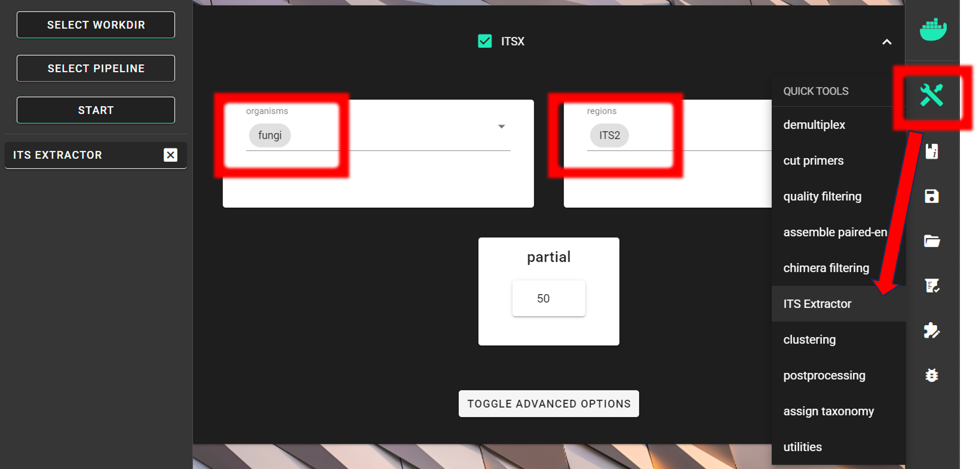
Since we are interesed only in fungi, we can limit the organisms to only fungi and keep the regions as ITS2. Universal ITS2 primers amplify also other eukaryotes besides fungi, thus, this step helps also to discard off-target sequences when limiting the organisms to only fungi. However, note that this increase in specificity may lead to some decrease in sensitivity; i.e., discarding some Fungal OTUs. For real-world applications, you may set organism to “all”, and discard off-target OTUs after the taxonomy assignment step.

Note

If you are working with only 5’-3’ oriented amplicons, then turn off complement setting under TOGGLE ADVANCE OPTIONS to skip the reverse complementary search; and possibly add more cores to speed things up (see here).

The partial setting is set to 50, which means that if at least one of the 5.8S or 28S motif is found in the sequence and that sequence is at least 50 bp long (after cutting the motif), then it will be classified as partial ITS2 sequence and outputted in the ITS2/full_and_partial directory.

Note

For better detection of the 18S, 5.8S and/or 28S regions by ITSx, you may not want to CUT PRIMERS in your own dataset. With this example dataset, ITSx works fine even when primers were clipped.

Input data

Via SELECT WORKDIR button, we specify the ASVs_out.dada2/curated directory as a working directory. The output directory, ITSx_out, will be created there (ASVs_out.dada2/curated/ITSx_out).

Automatically detected Sequence files extension may be .txt, but we need to set it to .fasta, so ITSx can work with the FASTA files in the working directory. The Sequencing read types do not matter here, just click ‘Confirm’.

Before starting ITSx

Note that all fasta files in the folder will be subjected to ITSx, so include to the WORKING DIRECTORY only ONE FASTA FILE within this workflow ASVs.fasta or ASVs_collapsed.fasta if there were any collapses with your own data.

The WORKING DIRECTORY can contain multiple FASTA files when the aim is to extract ITS2 sequences from all of them.

Outputs of ITSx

Output directory ITSx_out
ITS2/*.fasta	ITS2 sequences (without flanking gene fragments) per sample
ITS2/full_and_partial/*.fasta	full, but also partial ITS2 sequences per sample
seq_count_summary.txt	summary of sequence counts per sample

Checking the ITSx_out/ITS2/seq_count_summary.txt file, we see that ITS2 region was identified in all 21 ASVs.

File	Reads_in	Reads_out
ASVs.fasta	21	21

For the demonstration purposes, let’s examine the lenghts of the ASV sequences before and after ITSx:

Easy way to do this is to use seqkit stats tool (QuickTools --> Utilities).

seqkit stats output (seqkit_stats.fasta.txt):

File	format	type	num_seqs	sum_len	min_len	avg_len	max_len
ASVs.fasta	FASTA	DNA	21	6614	272	315.0	366
ASVs.ITS2.fasta	FASTA	DNA	21	4619	177	220.0	271

The sequences in the ASVs.fasta still contain the flanking 5.8S and LSU regions, while the sequences in the ASVs.ITS2.fasta only contain the ITS2 region. Therefore, the avg_len of the ASVs.ITS2.fasta is shorter than the avg_len of the ASVs.fasta.

The spread between min_len and max_len reflects true biological length variation of ITS2 among taxa.

Working with only ITS2 reads (without flanking gene fragments) may be useful as it standardizes what part of the rDNA amplicon you cluster (so clustering is driven by the ITS barcode region).

ITS2 ASVs

We can further proceed to cluster ASVs into OTUs, but if the aim is to work with ITS2 ASVs, then we need to match the ASV table to the ITS2 ASVs. In this example, ITSx did not remove any ASVs, therefore, the ASV table to work with is ASVs_table_TagJumpFilt.txt file in the ASVs_out.dada2/curated directory.

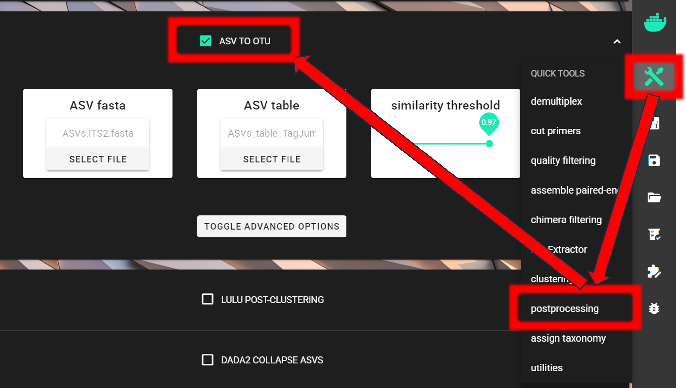
In case ITSx removed some ASVs, then you can use ASV TO OTU tool (QuickTools --> Postprocessing --> ASV TO OTU) with similarity threshold of 1 to match the input ASV table to the ITS2 ASVs. ASV TO OTU tool allows the ASVs in the input ASV fasta file to be a subset of the input ASV table.

Applying ASV TO OTU module with similarity threshold of 1 is the same thing as collapseNoMismatch = TRUE in the CURATE ASV TABLE process. It collapses identical ASVs by ignoring the end gaps, but if there are no identical ASVs, then it just matches the input ASV table to the ITS2 ASVs.

---

Cluster ASVs into OTUs

The ASVs approach may not accurately reflect species composition in the community of as fungi may have multiple different ITS copies per genome and may exhibit size polymorphism. Thus, here we aim to cluster the ASVs into OTUs (QuickTools --> Postprocessing --> ASV TO OTU).

Input fasta file is in the ITSx_out/ITS2/ASVs.ITS2.fasta and input ASV table is in the ASVs_out.dada2/curated/ASVs_table_TagJumpFilt.txt directory.

As a similarity threshold we are using the commonly used 97% (0.97, default setting).

Note

2nd column of the input ASV table must be ‘Sequences’ (1st column is ASV IDs; this is the default PipeCraft2 output table, so you don’t need to worry about this if you have followed this pipeline). For clustering, the ASV size annotation is obtained from the ASV table.

If the ASV table does not contain ‘Sequence’ column, then add those with QuickTools -> Utilities -> Add sequences to table see here.

Via SELECT WORKDIR button, we specify the ASVs_out.dada2/curated directory as a working directory (Sequence files extension and Sequencing read types do not matter here, just click ‘Confirm’).

The output directory, ASVs2OTUs_out, will be created there (ASVs_out.dada2/curated/ASVs2OTUs_out).

Outputs in ASVs2OTUs_out directory:
OTUs.fasta	FASTA formated representative OTU sequences
OTU_table.txt	OTU table (tab delimited file)
OTUs.uc	uclust-like formatted clustering results

---

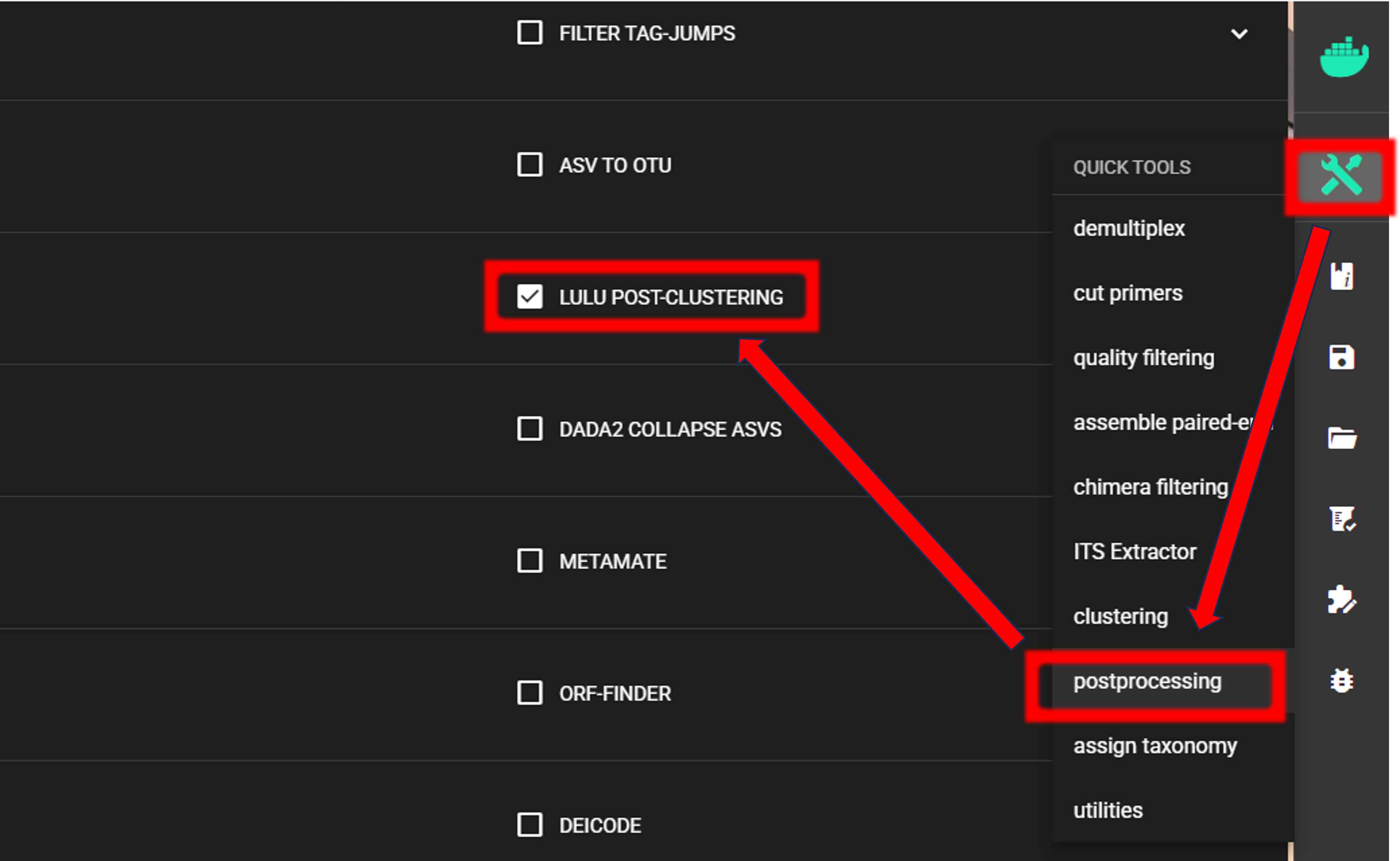
LULU post-clustering

Additionally, we can perform LULU post-clustering to merge co-occurring ‘daughter’ OTUs.

LULU description from the LULU repository: the purpose of LULU is to reduce the number of erroneous OTUs in OTU tables to achieve more realistic biodiversity metrics. By evaluating the co-occurence patterns of OTUs among samples LULU identifies OTUs that consistently satisfy some user selected criteria for being errors of more abundant OTUs and merges these. It has been shown that curation with LULU consistently result in more realistic diversity metrics.

Here, we are performing LULU post-clustering via QuickTools panel (on the right ribbon).

The input data are OTU_table.txt and OTUs.fasta files in the ASVs2OTUs_out directory. Here, we are using the default settings (which are suitable for most cases), but feel free to experiment with various settings to see the effect on the results.

To START

To START, specify working directory under SELECT WORKDIR (outputs will be written here), but the following requests about Sequence files extension and Sequencing read types do not matter here, just click ‘Confirm’.

The outputs of the process are in the lulu_out directory. But if we examine the README.txt file in that directory, then we see that “Total of 0 Features (OTUs/ASVs) were merged”, and therefore we do not have any OTU table or fasta file on the lulu_out folder. Note that this is a small example dataset, but with larger datasets postclustering merges many ‘daughter’ OTUs into ‘parent’ OTUs.

Thus, with this example dataset, our final OTU table and fasta file are OTU_table.txt and OTUs.fasta files in the ASVs2OTUs_out directory.

See this example of applying LULU post-clustering where LULU merged some OTUs.

---

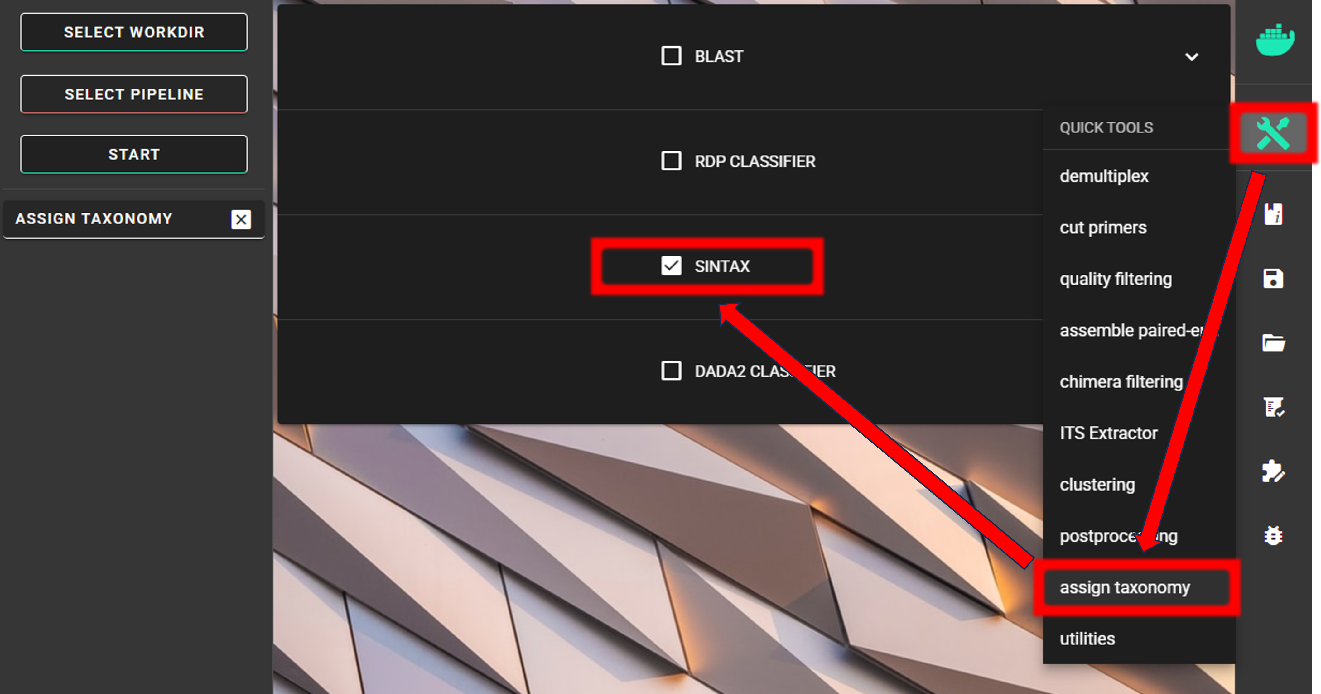
Assign taxonomy

Assign taxonomy is not the part of the full per-defined pipeline, but can be run as a separate step in QuickTools.

Here, we are using SINTAX. See other assign taxonomy options here.

We need to specify the location of the reference DATABASE for the taxonomic classification of our OTUs. For this example, we are using EUKARYOME database, which is a comprehensive database of eukaryotic ITS sequences; thus containing also other eukaryotic sequences besides Fungi. “Outgroups” are important in the reference database in order not to overclassify non-Fungal sequences as Fungi. Download the SINTAX_EUK_ITS file from here and unzip it (note: use 7-Zip software for unzipping files in Windows).

See other databases available for taxonomy annotation here.

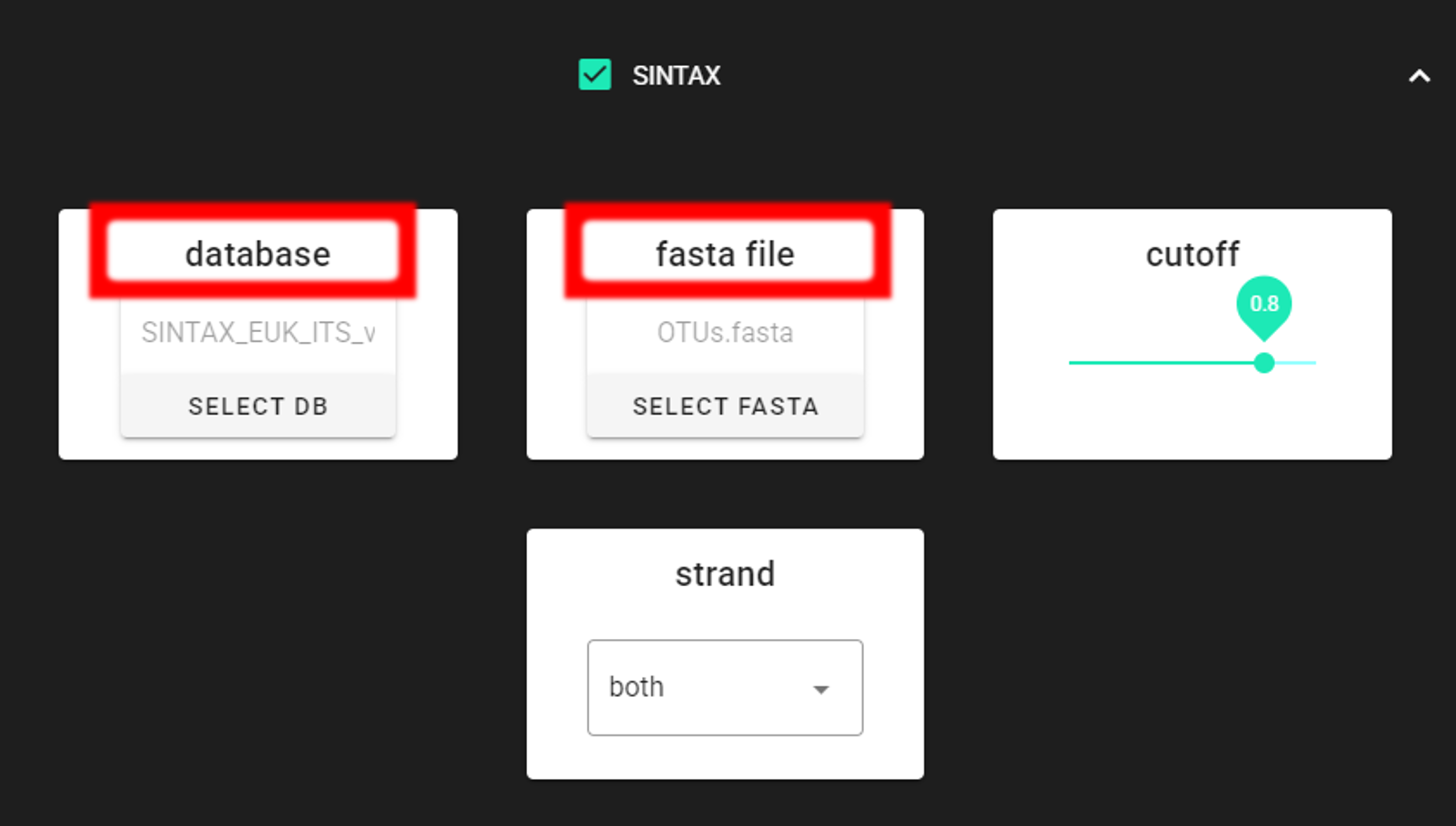
Specify the location of your downloaded database and also the fasta file with ASVs (fasta file) to be classified. Herein, we use OTUs.fasta file in the ASVs2OTUs_out directory (since we applied also ASV TO OTU process).

Important

Make sure you do not have any other SINTAX database files is the same directory as the database you are using. That is, use dedicated directory for the SINTAX database.

To START

To START, specify working directory under SELECT WORKDIR (outputs will be written here), but the following requests about Sequence files extension and Sequencing read types do not matter here, just click ‘Confirm’.

Note

First time usage of the fasta formatted database requires conversion to the SINTAX database format (.udb). This conversion is performed automatically by PipeCraft2, and will take some time, depending on the size of the database.

Result from the taxonomy annotation process - taxonomy table (taxonomy.sintax.txt) - is located at the taxonomy_out.sintax directory.

Output directory	taxonomy_out.sintax
taxonomy.sintax.txt	classifier results with bootstrap values

Taxonomy results for the first 4 OTUs

52f069d5552dbeaa8fe7dc379bd33c111bdc958f	d:Fungi(1.00),p:Basidiomycota(1.00),c:Agaricomycetes(1.00),o:Russulales(1.00),f:Albatrellaceae(1.00),g:Byssoporia(1.00),s:terrestris(0.53)	+	d:Fungi,p:Basidiomycota,c:Agaricomycetes,o:Russulales,f:Albatrellaceae,g:Byssoporia
99a50398b16a99aa01a932e3cfbf072c1313e8bd	d:Fungi(1.00),p:Basidiomycota(1.00),c:Agaricomycetes(1.00),o:Russulales(1.00),f:Russulaceae(1.00),g:Russula(1.00),s:chloroides(0.85)	+	d:Fungi,p:Basidiomycota,c:Agaricomycetes,o:Russulales,f:Russulaceae,g:Russula,s:chloroides
ed8775e608760e3c55fd15cf33eeed6690db89a2	d:Fungi(1.00),p:Ascomycota(1.00),c:Pezizomycetes(1.00),o:Pezizales(1.00),f:Pyronemataceae(1.00),g:Humaria(1.00),s:hemisphaerica(0.70)	+	d:Fungi,p:Ascomycota,c:Pezizomycetes,o:Pezizales,f:Pyronemataceae,g:Humaria
12a6e094e33bc2c9cf286bfde56fc73b90c26847	d:Fungi(1.00),p:Basidiomycota(1.00),c:Agaricomycetes(1.00),o:Russulales(1.00),f:Russulaceae(1.00),g:Lactarius(Fungi)(1.00)	+	d:Fungi,p:Basidiomycota,c:Agaricomycetes,o:Russulales,f:Russulaceae,g:Lactarius(Fungi)

taxonomy.sintax.txt is a tab-delimited text file without the initial header row:

• 1st column: OTU identifier (sha1 encoded)

• 2nd column: SINTAX classification result with bootstrap values in parentheses

• 3rd column: “+” sign

• 4th column: SINTAX classification result when considering the cutoff value (minimum bootstrap of 0.8)

In most cases, the 4th column of the taxonomy.sintax.txt is needed for further downstream ecological analyses. However, when using comma (,) as a field separator, the taxonomy in the 4th column has a variable number of fields (depending on the deepest rank SINTAX assigned at the cutoff).

Below, you can find a R-script to parse sintax taxonomy table (when EUKARYOME database is used). The R-script reads the SINTAX table, takes the 4th column, and writes taxonomy.sintax.formatted.txt with eight fixed columns for each rank. Missing ranks are filled with unclassified_<previous_rank> (for example, Species = unclassified_Lactarius when the deepest rank in column 4 is genus). EUKARYOME s: values are species epithets only; the script writes the binomial as Genus_epithet. Additional clarifications in genus names, specific to EUKARYOME database, such as Lactarius(Fungi) are reduced to Lactarius for the Genus and species columns.

For species level assignment, the R-script has an optional species_threshold argument, for requiring a higher bootstrap value for species assignment (stricter way for assigning species names.) When species_threshold in the script is set to 0.8 or higher, any row that has s: (species epithet) in the 4th column must also have a species assignment in the 2nd column with bootstrap ≥ species_threshold; otherwise the epithet is dropped and species name becomes unclassified_<Genus>. Set species_threshold to 0 to disable this check.

Parse taxonomy resulting from SINTAX run against EUKARYOME database

#!/usr/bin/env Rscript
### Format SINTAX column 4 for EUKARYOME.
### No-hit rows: all ranks output as "unclassified"

# specify input
taxtab <- "taxonomy.sintax.txt"

# (optional) species bootstrap filter: 0 = OFF.
species_threshold <- 0.9 # [allowed values: 0 or >= 0.8]

# specify output file name
outfile <- "taxonomy.sintax.formatted.txt"
#--------------------------------------#

# if running on CLI, use specified args
args <- commandArgs(trailingOnly = TRUE)
if (length(args) >= 1L) taxtab <- args[[1L]]
if (length(args) >= 2L) outfile <- args[[2L]]
if (length(args) >= 3L) species_threshold <- as.numeric(args[[3L]])

## Ranks in output order (used for NA fill and unclassified_* propagation)
TAX_RANKS <- c("Kingdom", "Phylum",
              "Class", "Order",
              "Family", "Genus",
              "Species")

## Strip trailing parenthetical qualifiers from genus
# when not a numeric bootstrap (e.g. Lactarius(Fungi)).
strip_genus_qualifier <- function(genus) {
  if (is.na(genus) || !nzchar(genus)) return(NA_character_)
  x <- sub("\\([^)]*[0-9][^)]*\\)$", "", genus)
  sub("\\([A-Za-z_][A-Za-z_ ]*\\)$", "", x)
}

## spaces -> underscores; empty -> NA.
sanitize_tokens <- function(x) {
  x <- trimws(as.character(x))
  keep <- !is.na(x) & nzchar(x)
  x[!keep] <- NA_character_
  x[keep] <- gsub("\\s+", "_", x[keep], perl = TRUE)
  x
}

## Species bootstrap from SINTAX column 2
extract_species_bootstrap <- function(col2_string) {
  s <- trimws(as.character(col2_string))
  if (is.na(s) || !nzchar(s)) return(NA_real_)
  m <- regmatches(s, regexec("s:[^(]+\\(([0-9.]+)\\)", s, perl = TRUE))[[1L]]
  if (length(m) < 2L) return(NA_real_)
  as.numeric(m[[2L]])
}

## No hits
is_no_hit_col4 <- function(s) {
  x <- trimws(as.character(s))
  is.na(x) | !nzchar(x) | x == "*"
}

## Parse one column-4 string into one row
parse_sintax_col4 <- function(s) {
  na_row <- function() {
    m <- matrix(
      NA_character_,
      nrow = 1L,
      ncol = 7L,
      dimnames = list(
        NULL,
        c("Kingdom", "Phylum",
          "Class", "Order",
          "Family", "Genus",
          "species_epithet")
      )
    )
    as.data.frame(m, stringsAsFactors = FALSE)
  }

  s <- trimws(as.character(s))
  if (is.na(s) || !nzchar(s) || s == "*") return(na_row())

  d_val <- k_val <- NA_character_
  row <- na_row()

  for (part in strsplit(s, ",", fixed = TRUE)[[1L]]) {
    part <- trimws(part)
    if (!nzchar(part) || !grepl("^[dkpcofgs]:", part)) next
    code <- substr(part, 1L, 1L)
    val <- substr(part, 3L, nchar(part))
    if (!nzchar(val)) next
    switch(code,
          "d" = { d_val <- val },
          "k" = { k_val <- val },
          "p" = { row$Phylum <- val },
          "c" = { row$Class <- val },
          "o" = { row$Order <- val },
          "f" = { row$Family <- val },
          "g" = { row$Genus <- val },
          "s" = { row$species_epithet <- val },
          NULL
    )
  }

  if (!is.na(k_val)) {
    row$Kingdom <- k_val
  } else if (!is.na(d_val)) {
    row$Kingdom <- d_val
  }
  row
}

replace_na_with_unclassified <- function(df) {
  out <- df
  km <- out[["Kingdom"]]
  out[["Kingdom"]] <- ifelse(is.na(km) | km == "",
                            "UnknownKingdom", km)
  for (i in 2L:length(TAX_RANKS)) {
    cur <- TAX_RANKS[i]
    prev <- TAX_RANKS[i - 1L]
    v <- out[[cur]]
    prev_v <- out[[prev]]
    out[[cur]] <- ifelse(is.na(v) | v == "",
                        paste0("unclassified_",
                                prev_v), v)
  }
  out
}

collapse_unclassified_prefix <- function(df) {
  out <- df
  for (nm in TAX_RANKS) {
    out[[nm]] <- gsub("^(unclassified_)+",
                      "unclassified_", out[[nm]],
                      perl = TRUE)
  }
  out
}

## Build Species = Genus_epithet where both present
species_binomial <- function(genus, epithet) {
  gen <- sanitize_tokens(genus)
  ep <- sanitize_tokens(epithet)
  ok <- !is.na(ep) & !is.na(gen)
  out <- rep(NA_character_, length(gen))
  out[ok] <- paste0(gen[ok], "_", ep[ok])
  out
}

## Load input and run parse
raw <- read.table(
  taxtab,
  sep = "\t",
  header = FALSE,
  stringsAsFactors = FALSE,
  quote = "",
  comment.char = "",
  fill = TRUE,
  check.names = FALSE
)

while (ncol(raw) < 4L) {
  raw <- cbind(raw, rep(NA_character_, nrow(raw)),
              stringsAsFactors = FALSE)
}

if (ncol(raw) < 1L || nrow(raw) < 1L) {
  stop("Expected at least one column and one row in ",
      taxtab)
}

feat_id <- as.character(raw[[1L]])
col4v <- as.character(raw[[4L]])
no_hit <- vapply(col4v, is_no_hit_col4, FUN.VALUE = NA)

parsed_df <- do.call(rbind, lapply(seq_len(nrow(raw)), function(i) {
  if (isTRUE(no_hit[i])) {
    data.frame(
      Kingdom = "unclassified",
      Phylum = "unclassified",
      Class = "unclassified",
      Order = "unclassified",
      Family = "unclassified",
      Genus = "unclassified",
      species_epithet = NA_character_,
      stringsAsFactors = FALSE
    )
  } else {
    parse_sintax_col4(col4v[i])
  }
}))
rownames(parsed_df) <- feat_id

parsed_df$Genus <- vapply(parsed_df$Genus,
                          strip_genus_qualifier,
                          FUN.VALUE = character(1L))

## species_threshold
st_num <- suppressWarnings(as.numeric(species_threshold))
if (!is.na(st_num) && st_num >= 0.8) {
  col2 <- as.character(raw[[2L]])
  sp_bt <- vapply(col2, extract_species_bootstrap, FUN.VALUE = NA_real_)
  epit <- parsed_df$species_epithet
  has_s4 <- !is.na(epit) & nzchar(trimws(as.character(epit)))
  fail <- !no_hit & has_s4 & (is.na(sp_bt) | sp_bt < st_num)
  parsed_df$species_epithet[fail] <- NA_character_
}

out <- data.frame(
  parsed_df[, c("Kingdom", "Phylum",
                "Class", "Order",
                "Family", "Genus"),
            drop = FALSE],
  Species = species_binomial(parsed_df$Genus,
                            parsed_df$species_epithet),
  stringsAsFactors = FALSE,
  row.names = rownames(parsed_df)
)

out <- replace_na_with_unclassified(out)
out <- collapse_unclassified_prefix(out)

## No-hit rows: every rank is "unclassified"
if (any(no_hit)) {
  ii <- which(no_hit)
  for (nm in TAX_RANKS) {
    out[ii, nm] <- "unclassified"
  }
}

out <- cbind(feature_id = feat_id, out,
            stringsAsFactors = FALSE)

# write output file
write.table(out, file = outfile,
            sep = "\t",
            quote = FALSE,
            row.names = FALSE,
            col.names = TRUE)

message("Wrote ", nrow(out), " rows to ", outfile)

You can copy-paste the script to a file and name it e.g., format_SINTAX_tax.R to run it on terminal (or run directly in RStudio).

 # Run with species_threshold of 0.9
 Rscript format_SINTAX_tax.R path/to/taxonomy.sintax.txt path/to/taxonomy.sintax.formatted.txt 0.9

# Run with species_threshold disabled
Rscript format_SINTAX_tax.R path/to/taxonomy.sintax.txt path/to/taxonomy.sintax.formatted.txt 0

The output file taxonomy.sintax.formatted.txt (with species_threshold of 0.9):

feature_id	Kingdom	Phylum	Class	Order	Family	Genus	Species
52f069d5552dbeaa8fe7dc379bd33c111bdc958f	Fungi	Basidiomycota	Agaricomycetes	Russulales	Albatrellaceae	Byssoporia	unclassified_Byssoporia
99a50398b16a99aa01a932e3cfbf072c1313e8bd	Fungi	Basidiomycota	Agaricomycetes	Russulales	Russulaceae	Russula	unclassified_Russula
ed8775e608760e3c55fd15cf33eeed6690db89a2	Fungi	Ascomycota	Pezizomycetes	Pezizales	Pyronemataceae	Humaria	unclassified_Humaria
12a6e094e33bc2c9cf286bfde56fc73b90c26847	Fungi	Basidiomycota	Agaricomycetes	Russulales	Russulaceae	Lactarius	unclassified_Lactarius