DADA2 ASVs pipeline, COI

This example dataset consists of COI mtDNA gene amplicon sequences with the target length of 313 bp:

Download example data set here and unzip it.

For this example data run, we are using a subset of CO1Classifier database in the taxonomy annotation process, download it from here.

---

Starting point

This example dataset consists of COI mtDNA gene amplicon sequences with the target length of 313 bp:

• paired-end Illumina MiSeq data;

• demultiplexed set (per-sample fastq files);

• primers are not not removed;

• sequences in this set are 5’-3’ (fwd) oriented.

when working with your own data …

… then please check that the paired-end data file names contain R1 and R2 strings (not just _1 and _2), so that PipeCraft can correctly identify the paired-end reads.

Example:

sample1_COI.R1.fq.gz

sample1_COI.R2.fq.gz

At least 2 samples (2x R1 + 2x R2 files) are required for this workflow! Otherwise ERROR in the denoising step:

---

To select DADA2 pipeline, press

SELECT PIPELINE –> DADA" ASVs.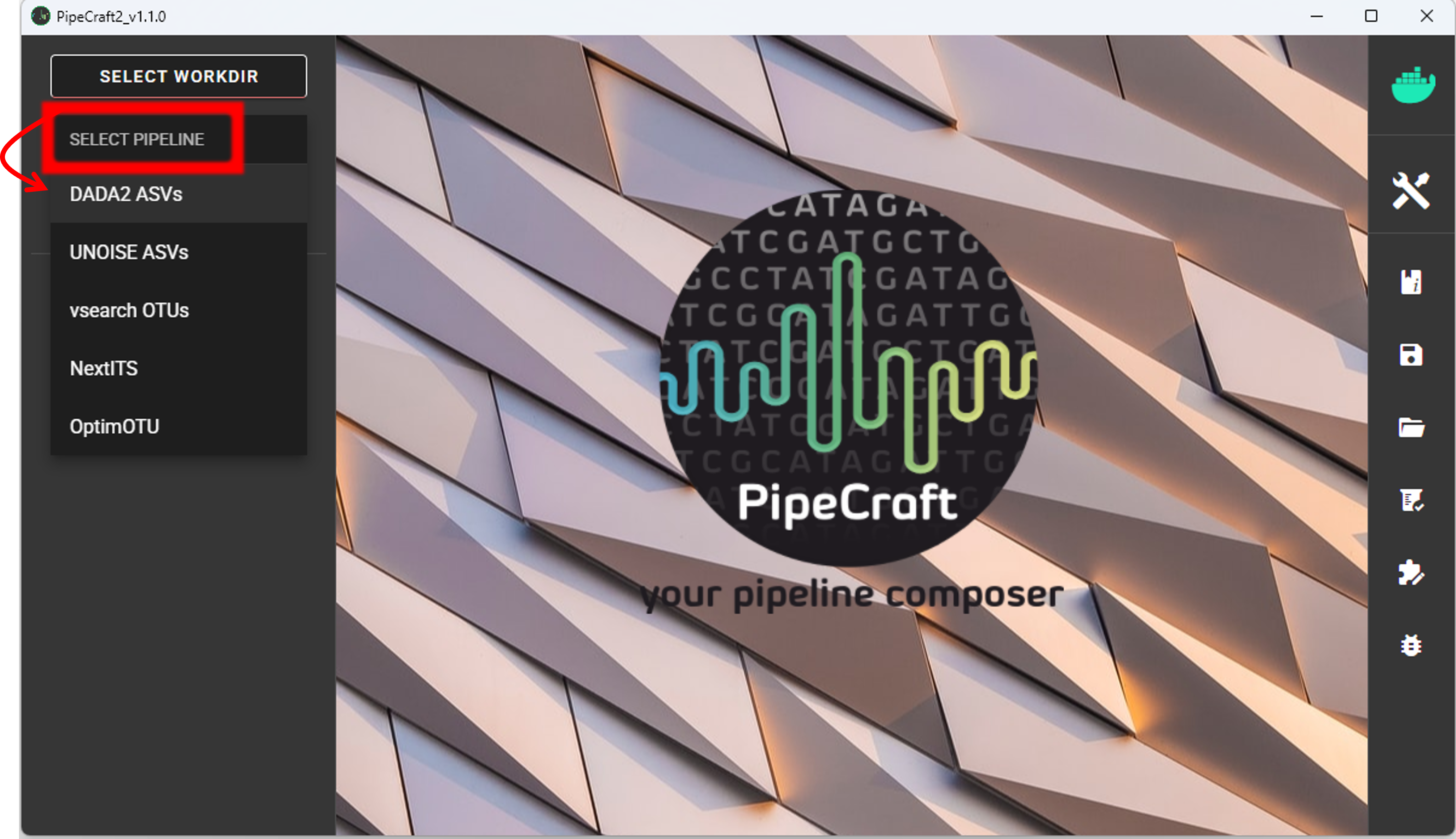

To select input data, press SELECT WORKDIR

and specify

sequence files extension as *.fastq;

sequencing read types as paired-end.

---

Workflow mode

Because we are working with sequences that are 5’-3’ oriented, we are selecting hte PAIRED-END FORWARD mode of the pipeline.

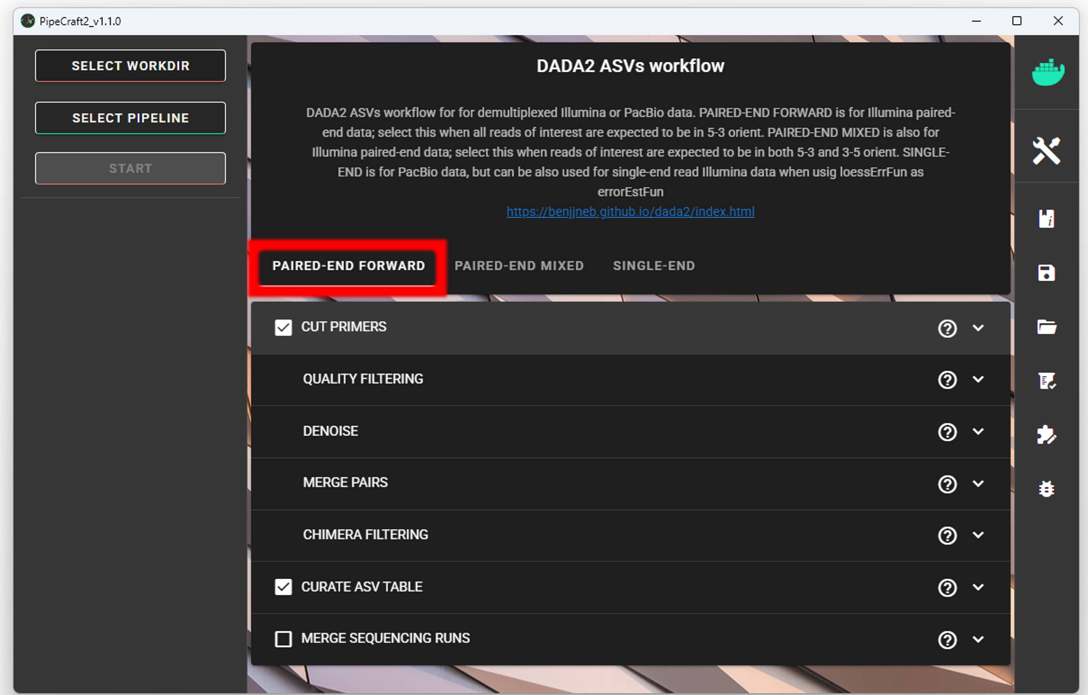
if sequences are in mixed orientation

If some sequences in your library are in 5’-3’ and some as 3’-5’ orientation, then with the ‘PAIRED-END FORWARD’ mode exactly the same ASV may be reported twice, where one ASV is just the reverse complementary of another. To avoid that, select PAIRED-END MIXED mode. Sequences have mixed orientation in libraries where sequenceing adapters have been ligated, rather than attached to amplicons during PCR.

Specifying primers (for CUT PRIMERS) is mandatory for the PAIRED-END MIXED mode. Based on the priemr sequences, the library will be split into two: 1) fwd oriented sequences, and 2) rev oriented sequences. Both batches are processed independently to produce ASVs, after which the rev oriented batch ASVs are reverse complemented and merged with the fwd oriented ASVs. Identical ASVs are merged to form a final data set. This is a reccomended workflow for accurate denoising compared with first reorienting all sequences to 5’-3’, and then performing a standard ‘PAIRED-END FORWARD’ workflow.

---

Cut primers

The example dataset contains primer sequences. Generally, we need to remove these to proceed the analyses only with the variable metabarcode of interest. If there are some additional sequence fragments, from eg. sequencing adapters or poly-G tails, then clipping the primers will remove those fragments as well.

Tick the box for CUT PRIMERS and specify forward and reverse primers. For the example data, the forward primer is GGWACWGGWTGAACWGTWTAYCCYCC and reverse primer is TANACYTCNGGRTGNCCRAARAAYCA.

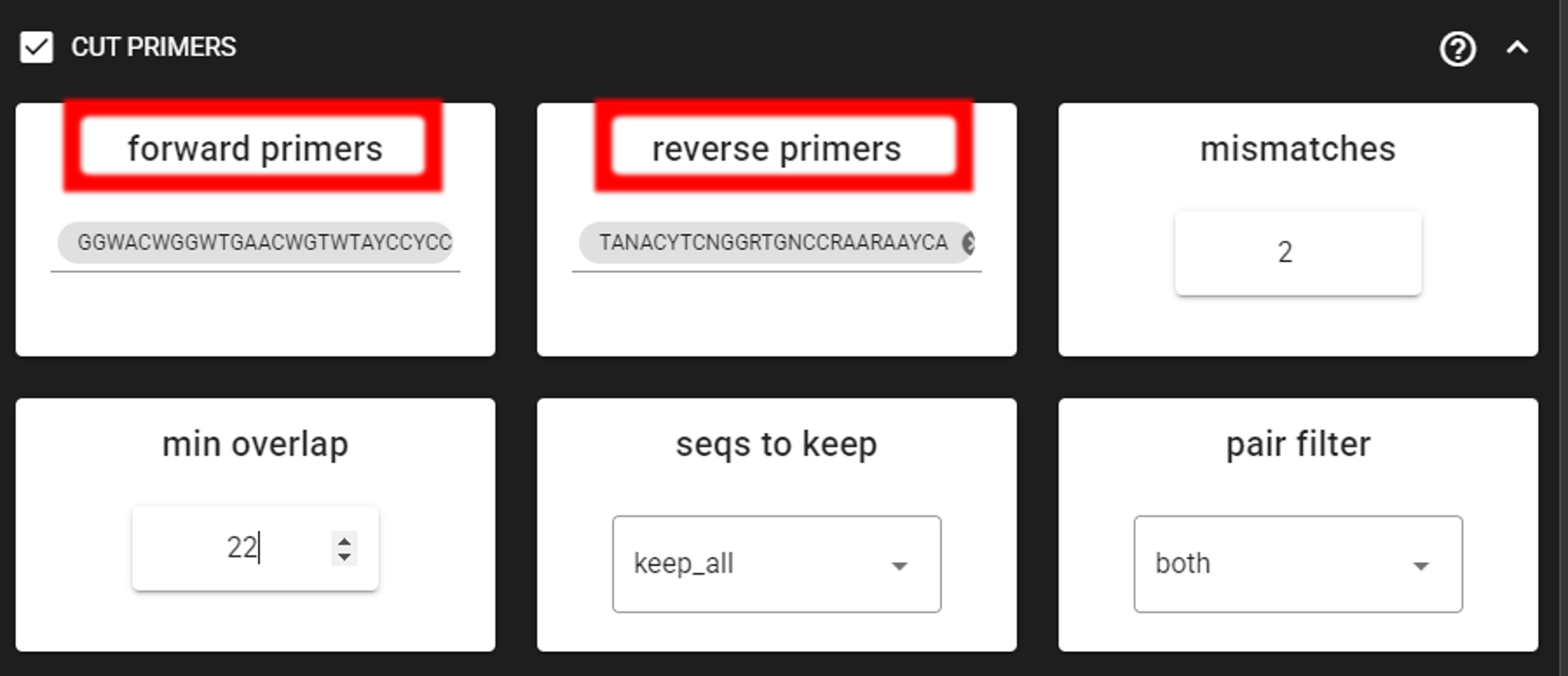
The primers are 26 bp - to keep a bit of flexibility in the primer search, we are requesting the min overlap of 22 bp and are allowing maximum of 2 mismatches . Note that too low min overlap may lead to random matches. Check other CUT PRIMER options here.

---

Quality filtering

Before adjusting quality filtering settings, let’s have a look on the quality profile of our example data set. Below quality profile plot was generated using QualityCheck panel (see here).

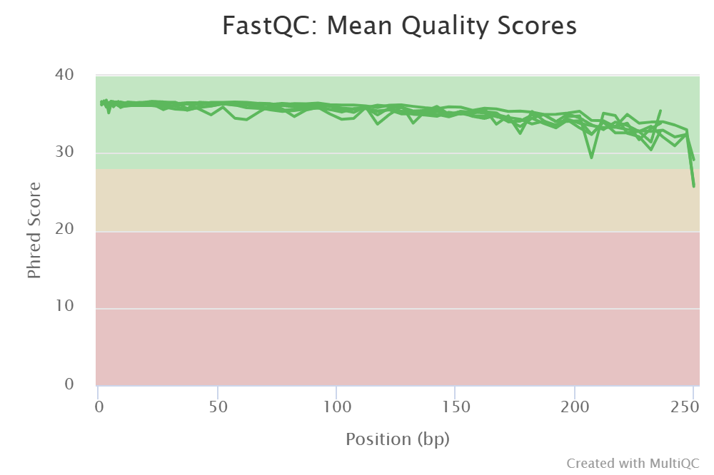
All files are represented with green lines, indicating good average quality per file (i.e., sample). However, if you see lower qualities of especially towards the end of R2 reads, then it not too alarming, since those can be clipped off with truncLen R2 setting (see remove low-quality ends/starts of reads section). DADA2 algoritm is robust to lower quality sequences, but removing the low quality read parts will improve the DADA2 sensitivity to rare sequence variants. But herein, we do not need to clip the ends, because the overall quality of the sequences is good enough.

---

Click on QUALITY FILTERING to expand the panel

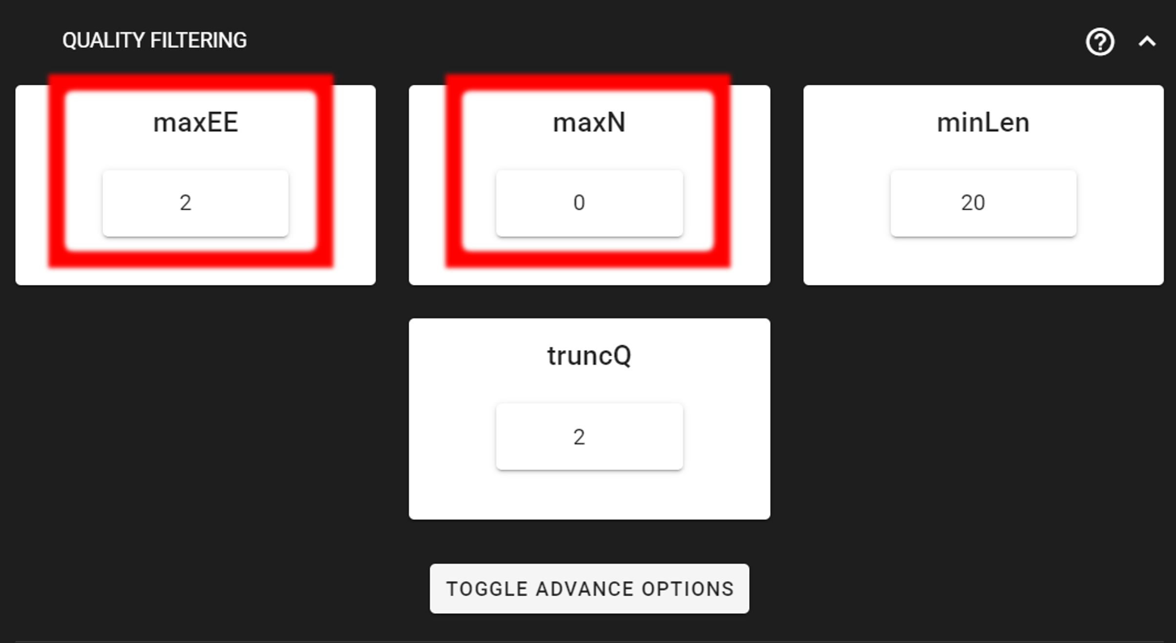
Here, we can leave the settings as DEFAULT by discarding sequences with maximum error rate of >2 and with ambiguous bases of >0.

Output directory qualFiltered_out
*.fq.gz	quality filtered sequences per sample in FASTQ format
*.rds	R objects for the following DADA2 workflow processes
seq_count_summary.csv	summary of sequence counts per sample

---

Denoise and merge pairs

This step performs desiosing (as implemented in DADA2), which first forms ASVs per R1 and R2 files. Then during merging/assembling process the paired ASV mates are assembled to output full amplicon length ASV.

Here, we are working with Illumina data, so let’s make sure that the errorEstFun setting is loessErrfun. We can leave all settings as DEFAULT.

Output directory denoised_assembled.dada2
*.fasta	denoised and assembled ASVs per sample in FASTA format
*.rds	R objects for the following DADA2 workflow processes
Error_rates_R*.pdf	plots for estimated R1/R2 error rates
seq_count_summary.csv	summary of sequence counts per sample

---

Chimera filtering

This step performs chimera filtering according to DADA2 removeBimeraDenovo function. During this step, the ASV table is also generated.

Important

make sure that primers have been removed from your amplicons; otherwise many false-positive chimeras may be filtered out from your dataset.

Here, we filter chimeras using the consensus method.

Output directory chimeraFiltered_out.dada2
*.fasta	chimera filtered ASVs per sample
seq_count_summary.csv	summary of sequence counts per sample
‘chimeras’ dir	ASVs per sample identified as chimeras

Output directory ASVs_out.dada2
ASVs_table.txt	denoised and chimera filtered ASV-by-sample table
ASVs.fasta	corresponding FASTA formated ASV Sequences
ASVs per sample identified as chimeras	rds formatted denoised and chimera filtered ASV table

---

Curate ASV table

This process first removes putative tag jumps and then collapses the ASVs that are identical up to shifts or length variation, i.e. ASVs that have no internal mismatches (PipeCraft2 uses vsearch usearch_global –id 1 for that); and finally filters out ASVs that are shorter/longer than specified length (in base pairs).

Here, we are enabling this process by checking the box for CURATE ASV TABLE in the DADA2 ASV workflow panel.

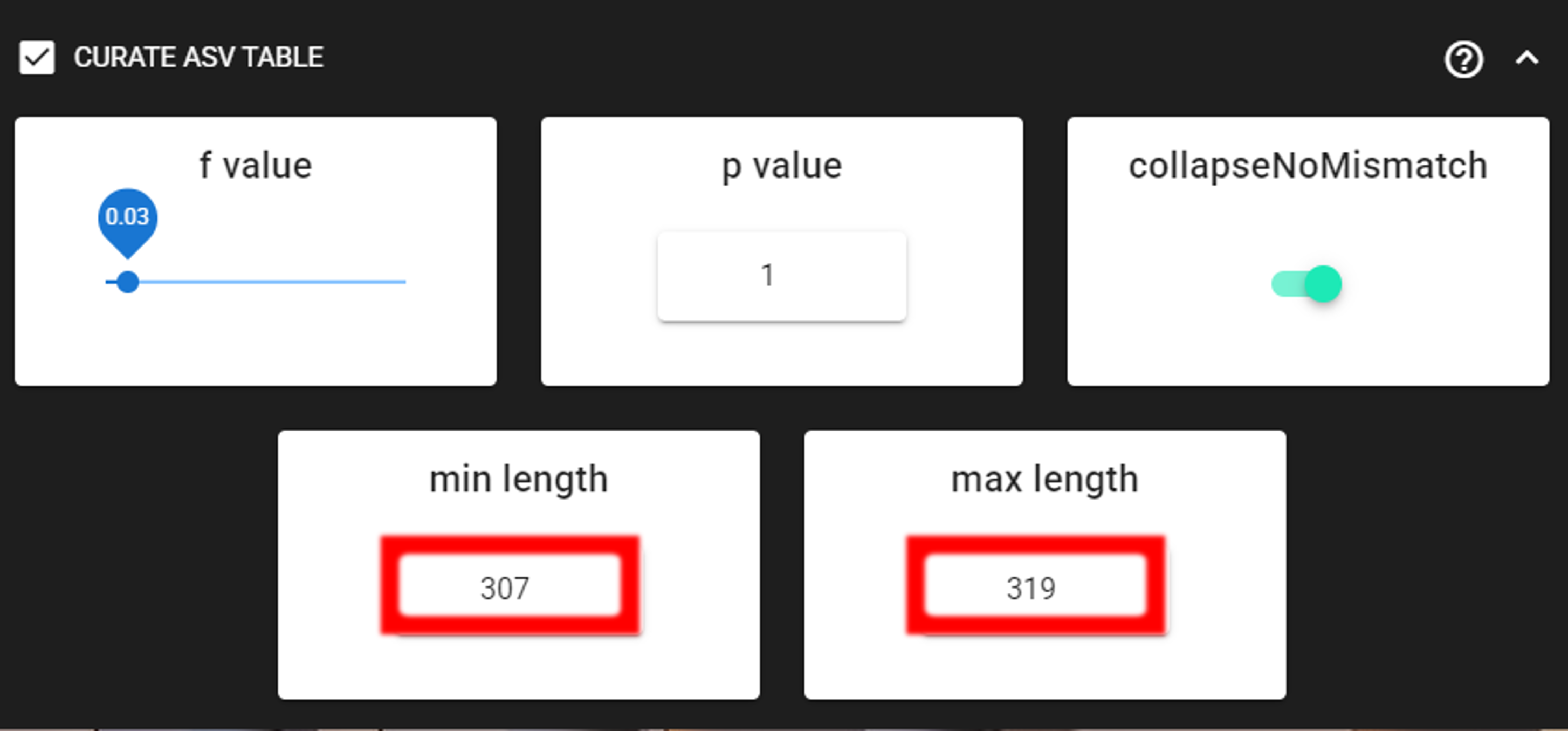
The f_value and p_value settings are used to filter out putative tag jumps (using UNCROSS2 algorithm). Generally, we recommend to use p_value of 1 (default), and f_value of 0.03 when using combinational indexing strategy; f_value of 0.05 when using single-indexes, and f_value of 0.01 when using unique dual-indexes.

The expected amplicon length (without primers) in our example dataset in 313 bp. Assuming that shorter sequences are non-target sequences, we use 307 in the min length setting and 319 in max length setting. This will discard ASVs that are shorter than 307 bp or longer than 319 bp.

We are also setting the collapseNoMismatch to TRUE, to collapse identical ASVs. This is basically equivalent to 100% clustering by ignoring the end gaps.

Output directory ASVs_out.dada2/curated
ASVs_table_TagJumpFilt.txt	only tag-jump filtered ASV-by-sample table
ASVs.fasta	corresponding ASV Sequences with ASVs_table_TagJumpFilt.txt table
ASVs_collapsed.fasta	tag-jump filtered and collapsed and size filtered ASV Sequences. Present only if some ASVs were collapsed.
ASVs_table_collapsed.txt	corresponding ASV-by-sample table. Present only if some ASVs were collapsed.
TagJump_stats.txt	summary of tag-jump filtering results

If there is nothing to collapse or filter out based on the length

then there are no corresponding files in the ASVs_out.dada2/curated directory, and only ASVs_table_TagJumpFilt.txt and ASVs.fasta files will be generated (even when there is nothing to tag-jump filter - in which case ASVs_table_TagJumpFilt.txt is the same ASVs_table.txt in the ASVs_out.dada2 directory).

Note

The pre-compiled pipeline ends here. Outputs COI ASVs should be further filtered to remove putative pseudogenes (NUMTs), and optionally ASVs can be clustered into OTUs. See below.

---

Save workflow

Once we have decided about the settings in our workflow, we can save the configuration file by pressing save workflow button on the right-ribbon

If you forget the save, then no worries, a pipecraft2_last_run_configuration.json file will be generated for you upon starting the workflow. As the file name says, it is the workflow configuration file for your last PipeCraft run in this working directory. If the file name (pipecraft2_last_run_configuration.json) is not changed, then the file is overwritten with the new configuration if running a new job in the same working directory.

This JSON file can be loaded into PipeCraft2 to automatically configure your next runs exactly the same way.

Note

‘Assign taxonomy’ is not the part of the full per-defined pipeline. This step can be selected and run via QuickTools panel. See below.

---

Start the workflow

Press START on the left ribbon to start the analyses.

when running the module for the first time …

… a docker image will be first pulled to start the process.

For example:

When you need to STOP the workflow, press STOP button

When the workflow has completed …

… a message window will be displayed.

---

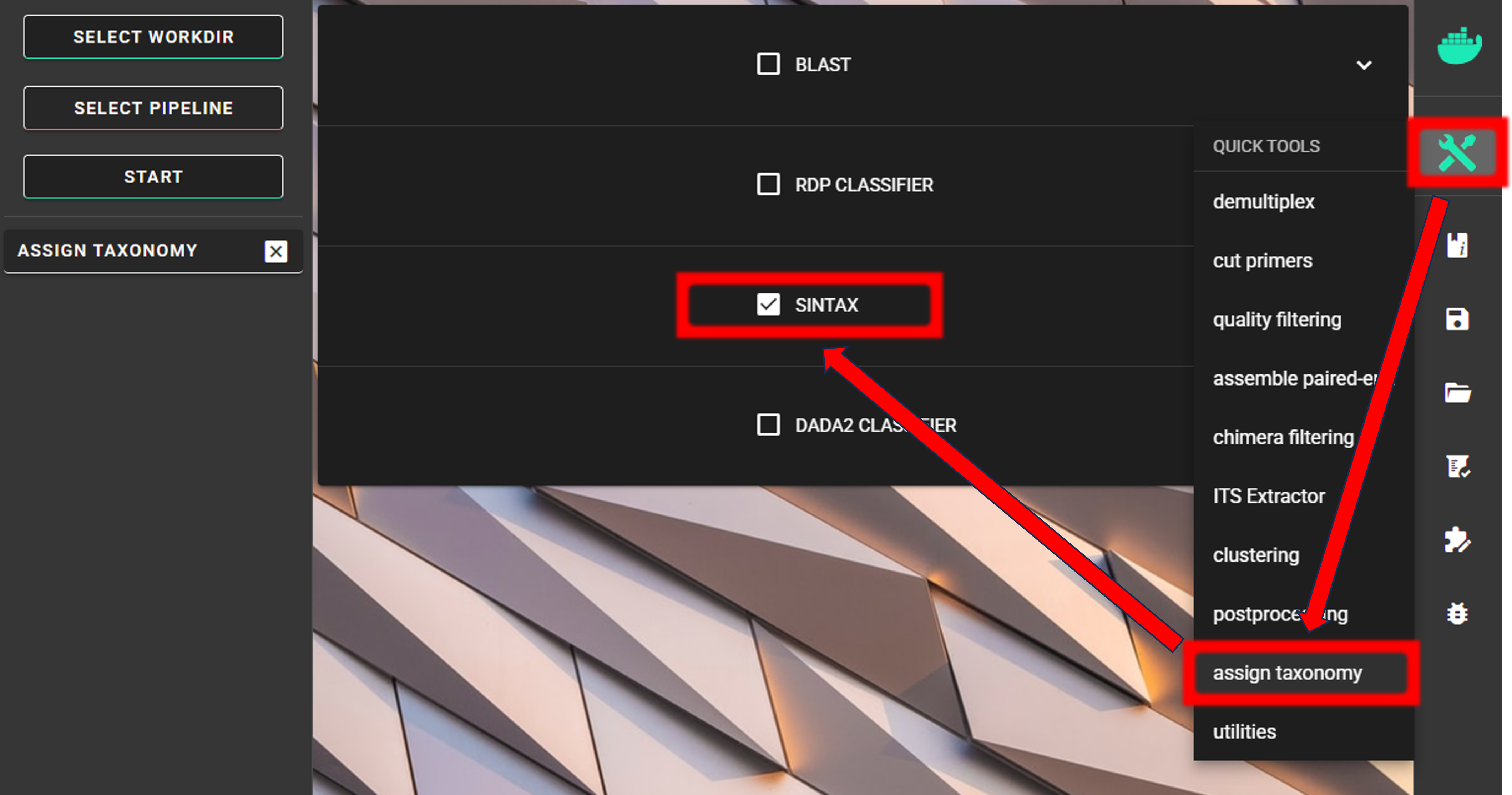
Assign taxonomy

Assign taxonomy is not the part of the full per-defined pipeline, but can be run as a separate step in QuickTools. Here, we are using the SINTAX classifier for that.

We need to specify the location of the reference DATABASE for the taxonomic classification of our ASVs. For this example data run, we are using a subset of CO1Classifier database in the taxonomy annotation process, download it from here

Specify the location of your downloaded database and also the fasta file with ASVs (fasta file) to be classified. Herein, we use ASVs_collapsed.fasta file in the ASVs_out.dada2/curated directory (since we applied also CURATE ASV TABLE process (see below Examine the outputs section)).

We can use the default cutoff (minimum bootstrap; ranging from 0-1; ~assignment confidence) value of 0.8. This means that taxonomic ranks with at least bootstrap value of 80 will get classification (unclassified for <0.8).

strand may be plus (since we are expecting only 5’-3’ oriented ASVs), but since SINTAX is fast, I’ll leave it as default (both - comparre both strands).

To START

To START, specify working directory under SELECT WORKDIR (outputs will be written here), but the following requests about Sequence files extension and Sequencing read types do not matter here, just click ‘Confirm’.

Note

First time usage of the fasta formatted database requires conversion to the SINTAX database format (.udb). This conversion is performed automatically by PipeCraft2, and will take some time, depending on the size of the database.

Output directory	taxonomy_out.sintax
taxonomy.sintax.txt	classifier results with bootstrap values

---

Examine the outputs

Several process-specific output folders are generated

primersCut_out	paired-end fastq files per sample, primers clipped
qualFiltered_out	quality filtered paired-end fastq files per sample
denoised_assembled.dada2	denoised and assembled fasta files per sample
chimeraFiltered_out.dada2	chimera filtered fasta files per sample
ASVs_out.dada2	ASVs table, and ASV sequences files
ASVs_out.dada2/curated	curated ASVs table, and ASV sequences files
taxonomy_out.dada2	ASVs taxonomy table (taxonomy.csv)

Each folder (except ASVs_out.dada2 and taxonomy_out.dada2) contain summary of the sequence counts (seq_count_summary.csv). Examine those to track the read counts throughout the pipeline.

For example, from the seq_count_summary.csv file in qualFiltered_out we see that most of the sequences survived the quality filtering step. The input column represents the number of input sequences for the quality filtering step (that is, sequences from CUT PRIMERS step); the qualFiltered column represents the number of sequences that survived the quality filtering step.

	input	qualFiltered
sample1_COI	999	830
sample2_COI	999	829
sample3_COI	999	871

---

Final outputs of the pipeline

Here, we applied also “CURATE ASV TABLE” process. Therefore, our final outputs of the pipeline are in the ASVs_out.dada2/curated directory, which contans:

ASVs_table_TagJumpFilt.txt	only tag-jump filtered ASV-by-sample table
ASVs.fasta	corresponding ASV Sequences with ASVs_table_TagJumpFilt.txt table
ASVs_collapsed.fasta	tag-jump filtered and collapsed and size filtered ASV Sequences.
ASVs_table_collapsed.txt	corresponding ASV-by-sample table.
TagJump_stats.txt	summary of tag-jump filtering results

Important

COI amplicons should be also checked for the presence of putative pseudogenes (NUMTs). (see below Remove NUMTs section)).

If we see the ASVs_table_collapsed.txt in the ASVs_out.dada2/curated directory, then this means that some ASVs were collapsed and/or discarded because of the length filtering.

Let’s check the README.txt file: there we can read that input ASV table (ASVs_out.dada2/ASVs_table.txt) had 27 ASVs and the output ASVs table (ASVs_out.dada2/curated/ASVs_table_collapsed.txt) had 23 ASVs. Further, it says that lenFilt resulted in 23 Features (ASVs). This means that 4 ASVs were discarded because of the length filtering not because some were collapsed.

The length filtering and collapsing has been performed upon tag-jump filted ASV table (ASVs_table_TagJumpFilt.txt), therefore, the final outputs of the pipeline are ASVs_table_collapsed.txt and ASVs_collapsed.fasta

ASVs_table_collapsed.txt represents the ASV table after the tag-jump and lenght/collapse filtering, where the 1st column represents ASV identifiers (sha1 encoded), 2nd column is the sequence of an ASV, and all the following columns represent number of sequences in the corresponding samples (sample name is taken from the file name). This is tab delimited text file.

ASVs_table_collapsed.txt:

OTU	Sequence	sample1_COI	sample2_COI	sample3_COI
e837216e5…	TTTATCTT…	0	0	682
46a9fb279…	ACTATCCTC…	583	0	0
37838deee…	TTAGCAGGG..	0	342	0
c787bfb1f…	TCTTGCAA…	215	0	0

Note: even though the ASVs column header is “OTU”, it represents ASVs as we preformed an ASVs workflow!

We applied also tag-jump filtering process (via f_value and p_value settings). When checking the TagJump_stats.txt file in the ASVs_out.dada2/curated directory, we see that based on our settings, 0 tag-jump events were detected. [Therefore, ASVs_table_TagJumpFilt.txt and ASVs_out.dada2/ASVs_table.txt files are the same.]

---

Result from the taxonomy annotation process - taxonomy table (taxonomy.sintax.txt) - is located at the taxonomy_out.sintax directory.

Taxonomy results for the first 4 ASVs

24a03fcd59d40823dcc5aacb594e9fc6b68bcf6b	d:Eukaryota(1.00),k:Metazoa(1.00),p:Arthropoda(0.97),c:Insecta(0.31),o:Coleoptera(0.26),f:Curculionidae(0.17),g:Laparocerus(0.17),s:Laparocerus_exiguus(0.09)	+	d:Eukaryota,k:Metazoa,p:Arthropoda
46a9fb279afe3d45b304409d09d63e9181f94096	d:Eukaryota(1.00),k:Metazoa(1.00),p:Arthropoda(1.00),c:Chilopoda(1.00),o:Lithobiomorpha(1.00),f:Lithobiidae(1.00),g:Lithobius(1.00),s:Lithobius_curtipes(1.00)	+	d:Eukaryota,k:Metazoa,p:Arthropoda,c:Chilopoda,o:Lithobiomorpha,f:Lithobiidae,g:Lithobius,s:Lithobius_curtipes
c787bfb1fb95d92352fe1579dcc1a8f67c0d5ebe	d:Eukaryota(1.00),k:Metazoa(1.00),p:Annelida(1.00),c:Clitellata(1.00),o:Enchytraeida(1.00),f:Enchytraeidae(1.00),g:Fridericia_segmented_worms(1.00),s:Fridericia_eiseni(0.99)	+	d:Eukaryota,k:Metazoa,p:Annelida,c:Clitellata,o:Enchytraeida,f:Enchytraeidae,g:Fridericia_segmented_worms,s:Fridericia_eiseni
e837216e5c192a25cf3808ba39f29c34b3fe00e9	d:Eukaryota(1.00),k:Metazoa(0.93),p:Arthropoda(0.92),c:Insecta(0.52),o:Lepidoptera(0.26),f:Geometridae(0.09),g:Homospora(0.06),s:Homospora_rhodoscopa(0.06)	+	d:Eukaryota,k:Metazoa,p:Arthropoda

taxonomy.sintax.txt is a tab-delimited text file without the initial header row:

• 1st column: ASV identifier (sha1 encoded)

• 2nd column: SINTAX classification result with bootstrap values in parentheses

• 3rd column: “+” sign

• 4th column: SINTAX classification result when considering the cutoff value (minimum bootstrap of 0.8)

---

Check for the non-target hits

It is often the case that universal metabarcoding primers amplify also non-target DNA regions and/or non-target taxa. Working with this example dataset, we are interesed only in Metazoa (Animals), thus we should get rid of the off-target noise before proceeding with relevant statistical analyses.

When we carefully examine the results, the taxonomy table, then we can see that 1 ASV is classifed to Fungi, 1 ASVs is unclassified to kingdom level (kingdom le). But even among the Metazoa, there are some off-target hits; 1 ASV is classified as Chordata (specifically as Homo sapiens, human). We are not interested in latter as well. We should remove all of those off-target ASVs.

Below, you can find a R script to clean and organize sintax taxonomy table, as well as clean ASV table and ASVs fasta file from the off-target taxa.

Clean and organize sintax taxonomy table, as well as clean ASV table and ASVs fasta file from the off-target taxa

#!/usr/bin/env Rscript
### Filter dataset based on SINTAX results to include target taxa

# specify taxon and threshold
target="Metazoa"            # target taxonomic group(s);
                            # multiple groups should be from the same taxonomic level
                            # separator is "," (e.g., "Hymenoptera, Lepidoptera")
tax_level="kingdom"         # allowed levels: kingdom | phylum | class | order | family | genus
off_targets = c("Chordata") # a list of off-targets within target
threshold="0.8"             # threshold for considering an ASV as a target taxon
species_threshold = 0.9     # threshold for species level identification

# specify the ASV table and ASVs.fasta file that would be filtered to include only target taxa
ASV_fasta = "ASVs_collapsed.fasta"
ASV_table = "ASVs_table_collapsed.txt"

# specify the SINTAX-classifier output file (taxonomy file)
taxtab="taxonomy.sintax.txt"

#--------------------------------------#
library(stringr)
library(dplyr)
library(Biostrings)

# Function to parse SINTAX taxonomy format from vsearch output
parse_sintax = function(tax_string) {
  # Initialize result with NAs
  result = list(
    kingdom = NA, kingdom_conf = 0,
    phylum = NA, phylum_conf = 0,
    class = NA, class_conf = 0,
    order = NA, order_conf = 0,
    family = NA, family_conf = 0,
    genus = NA, genus_conf = 0,
    species = NA, species_conf = 0
  )

  if (is.na(tax_string) || tax_string == "" || tax_string == "*") {
    return(result)
  }

  # Split by comma
  ranks = strsplit(tax_string, ",")[[1]]

  for (rank in ranks) {
    # Extract rank prefix (d:, k:, p:, c:, o:, f:, g:, s:)
    if (grepl("^d:", rank)) {
      # Domain (skip, not used)
      next
    } else if (grepl("^k:", rank)) {
      # Kingdom
      match = regmatches(rank, regexec("k:([^(]+)\\(([0-9.]+)\\)", rank))[[1]]
      if (length(match) == 3) {
        result$kingdom = match[2]
        result$kingdom_conf = as.numeric(match[3])
      }
    } else if (grepl("^p:", rank)) {
      # Phylum
      match = regmatches(rank, regexec("p:([^(]+)\\(([0-9.]+)\\)", rank))[[1]]
      if (length(match) == 3) {
        result$phylum = match[2]
        result$phylum_conf = as.numeric(match[3])
      }
    } else if (grepl("^c:", rank)) {
      # Class
      match = regmatches(rank, regexec("c:([^(]+)\\(([0-9.]+)\\)", rank))[[1]]
      if (length(match) == 3) {
        result$class = match[2]
        result$class_conf = as.numeric(match[3])
      }
    } else if (grepl("^o:", rank)) {
      # Order
      match = regmatches(rank, regexec("o:([^(]+)\\(([0-9.]+)\\)", rank))[[1]]
      if (length(match) == 3) {
        result$order = match[2]
        result$order_conf = as.numeric(match[3])
      }
    } else if (grepl("^f:", rank)) {
      # Family
      match = regmatches(rank, regexec("f:([^(]+)\\(([0-9.]+)\\)", rank))[[1]]
      if (length(match) == 3) {
        result$family = match[2]
        result$family_conf = as.numeric(match[3])
      }
    } else if (grepl("^g:", rank)) {
      # Genus
      match = regmatches(rank, regexec("g:([^(]+)\\(([0-9.]+)\\)", rank))[[1]]
      if (length(match) == 3) {
        result$genus = match[2]
        result$genus_conf = as.numeric(match[3])
      }
    } else if (grepl("^s:", rank)) {
      # Species
      match = regmatches(rank, regexec("s:([^(]+)\\(([0-9.]+)\\)", rank))[[1]]
      if (length(match) == 3) {
        result$species = match[2]
        result$species_conf = as.numeric(match[3])
      }
    }
  }

  return(result)
}

# read ASV table
table = read.table(ASV_table, sep = "\t", check.names = F, header = T, row.names = 1)

# read SINTAX taxonomy table (vsearch --sintax output format)
# Format: ASV_ID \t taxonomy_string \t strand \t other_columns
tax_raw = read.table(taxtab, sep = "\t", check.names = F, header = F,
                    stringsAsFactors = F, quote = "", comment.char = "", fill = TRUE)

# Take first two columns only (ASV_ID and taxonomy)
tax_raw = tax_raw[, 1:2]
colnames(tax_raw) = c("ASV", "taxonomy")
rownames(tax_raw) = tax_raw$ASV

cat("\n Input =", nrow(tax_raw), "features.\n")

# Parse SINTAX taxonomy strings
tax_list = lapply(tax_raw$taxonomy, parse_sintax)
tax = do.call(rbind, lapply(tax_list, as.data.frame))
rownames(tax) = tax_raw$ASV

# taxon list
taxon_list = strsplit(target, ", ")[[1]]

### extract only target-taxon ASVs from the 'raw' SINTAX results
tax_filtered = tax %>%
  filter(.data[[tax_level]] %in% taxon_list)

cat("\n Found", nrow(tax_filtered), "ASVs matching", target, "at", tax_level, "level.\n")

### change all tax ranks to "unclassified_*" when
# the confidence values is less than the specified threshold
# kingdom
tax_filtered = tax_filtered %>%
  mutate(kingdom = ifelse(kingdom_conf < threshold | is.na(kingdom),
                          "unclassified_root", as.character(kingdom)))

# phylum
tax_filtered = tax_filtered %>%
  mutate(phylum = ifelse(phylum_conf < threshold | is.na(phylum),
                        paste0("unclassified_", kingdom), as.character(phylum)))
tax_filtered$phylum = stringr::str_replace(tax_filtered$phylum, "unclassified_unclassified_",
                                          "unclassified_")

# class
tax_filtered = tax_filtered %>%
  mutate(class = ifelse(class_conf < threshold | is.na(class),
                        paste0("unclassified_", phylum), as.character(class)))
tax_filtered$class = stringr::str_replace(tax_filtered$class, "unclassified_unclassified_",
                                          "unclassified_")

# order
tax_filtered = tax_filtered %>%
  mutate(order = ifelse(order_conf < threshold | is.na(order),
                        paste0("unclassified_", class), as.character(order)))
tax_filtered$order = stringr::str_replace(tax_filtered$order, "unclassified_unclassified_",
                                          "unclassified_")

# family
tax_filtered = tax_filtered %>%
  mutate(family = ifelse(family_conf < threshold | is.na(family),
                        paste0("unclassified_", order), as.character(family)))
tax_filtered$family = stringr::str_replace(tax_filtered$family, "unclassified_unclassified_",
                                          "unclassified_")

# genus
tax_filtered = tax_filtered %>%
  mutate(genus = ifelse(genus_conf < threshold | is.na(genus),
                        paste0("unclassified_", family), as.character(genus)))
tax_filtered$genus = stringr::str_replace(tax_filtered$genus, "unclassified_unclassified_",
                                          "unclassified_")

# species to genus_sp when the confidence values is < species_threshold
tax_filtered = tax_filtered %>%
  mutate(species = ifelse(species_conf < species_threshold | is.na(species),
                          paste0(genus, "_sp"), as.character(species)))

### exclude off-target taxa at any taxonomic level
if (length(off_targets) > 0 && !all(is.na(off_targets)) && off_targets[1] != "") {
  # Count ASVs before exclusion
  n_before_exclusion = nrow(tax_filtered)

  # Exclude ASVs where any taxonomic level matches off-targets
  # Check all taxonomic ranks: kingdom, phylum, class, order, family, genus, species
  tax_filtered = tax_filtered %>%
    filter(!(kingdom %in% off_targets |
            phylum %in% off_targets |
            class %in% off_targets |
            order %in% off_targets |
            family %in% off_targets |
            genus %in% off_targets |
            species %in% off_targets))

  n_after_exclusion = nrow(tax_filtered)
  n_excluded = n_before_exclusion - n_after_exclusion

  cat("\n Excluded", n_excluded, "ASVs matching off-target taxa at any taxonomic level:",
                                              paste(off_targets, collapse = ", "), "\n")
  cat(" Remaining ASVs after exclusion:", n_after_exclusion, "\n")
}

### count occurrences of each taxon in df (SINTAX results)
count_taxa = function(df, taxa) {
  sapply(taxa, function(taxon) sum(apply(df, 1, function(row) any(row == taxon))))
}
taxon_counts = count_taxa(tax_filtered, taxon_list)

# Check the counts
if (all(taxon_counts == 0)) {
  print("ERROR: None of the specified taxa are present in the SINTAX results.")
} else {
  if (any(taxon_counts == 0)) {
    warning("One or more of the specified taxa are not present in the SINTAX results.")
  }
  cat("\n Taxon counts:\n")
  print(taxon_counts)
}

### extract only target-taxon ASVs from the 'threshold filtered' SINTAX results
tax_filtered_thresh = tax_filtered %>%
  filter(.data[[tax_level]] %in% taxon_list)

# Remove confidence columns for output
tax_filtered_output = tax_filtered_thresh %>%
  select(kingdom, phylum, class, order, family, genus, species)

# write filtered SINTAX taxonomy table
tax_filtered_output = cbind(ASV = rownames(tax_filtered_output), tax_filtered_output)
write.table(tax_filtered_output,
            file = "taxonomy.sintax.filt.txt",
            quote = F,
            row.names = F,
            sep = "\t")

### filter the ASV table to match ASVs that were kept in the tax_filtered table
table_filt = table[rownames(table) %in% rownames(tax_filtered_thresh), ]

# write filtered table
table_filt = cbind(ASV = rownames(table_filt), table_filt)
write.table(table_filt,
            file = paste0(sub("\\.[^.]*$", "_tax_filt.txt", ASV_table)),
            quote = F,
            row.names = F,
            sep = "\t")

# filter ASV_fasta
fasta = readDNAStringSet(ASV_fasta)
fasta.tax_filt = fasta[names(fasta) %in% rownames(table_filt)]

# write filtered ASV_fasta
writeXStringSet(fasta.tax_filt,
                paste0(sub("\\.[^.]*$", "_tax_filt.fasta", ASV_fasta)),
                width = max(width(fasta.tax_filt)))

Output files where off-target taxa have been removed:

• taxonomy.sintax.filt.txt: filtered SINTAX taxonomy table

• ASVs_table_collapsed_tax_filt.txt: taxonomy filtered ASV table

• ASVs_collapsed_tax_filt.fasta: taxonomy filtered ASVs fasta file

Example of the filtered SINTAX taxonomy table:

ASV	kingdom	phylum	class	order	family	genus	species
46a9fb279afe3d45b304409d09d63e9181f94096	Metazoa	Arthropoda	Chilopoda	Lithobiomorpha	Lithobiidae	Lithobius	Lithobius_curtipes
37838deee5cc9233c9ac7c74f01d8c06a7912bb1	Metazoa	Arthropoda	Arachnida	Sarcoptiformes	Liacaridae	Adoristes	Adoristes_ovatus
c787bfb1fb95d92352fe1579dcc1a8f67c0d5ebe	Metazoa	Annelida	Clitellata	Enchytraeida	Enchytraeidae	Fridericia_segmented_worms	Fridericia_eiseni
e837216e5c192a25cf3808ba39f29c34b3fe00e9	Metazoa	Arthropoda	unclassified_Arthropoda	unclassified_Arthropoda	unclassified_Arthropoda	unclassified_Arthropoda	unclassified_Arthropoda_sp

Note that the taxonomix ranks with lower bootstrap values than ``cutoff`` value have been changed to “unclassified_”.*

---

Additional processes via QuickTools

The following are additional steps that can be performed, with removing putative NUMTs as the most important one for COI data.

---

Remove NUMTs

When working with processing protein-coding markers (such as COI), the amplified sequences of nuclear mitochondrial pseudogenes (NUMTs) may inflate the richness estimates and thus introduce biases in biodiversity research using metabarcoding. Therefore, it is important to remove these sequences from the data set.

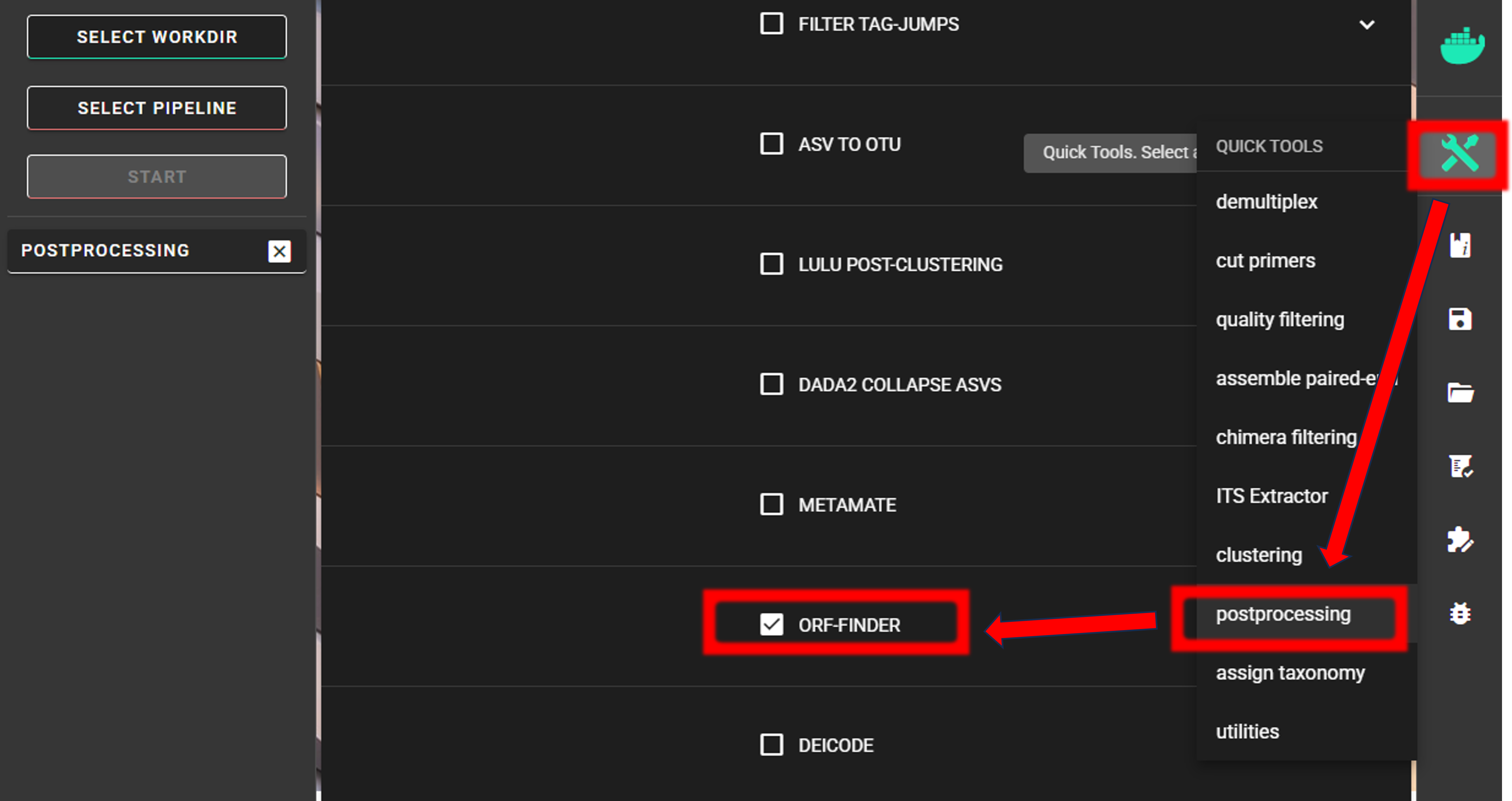
In PipeCraft2, there are tools such as metaMATE and ORFfinder that can be used to remove NUMTs from the data set.

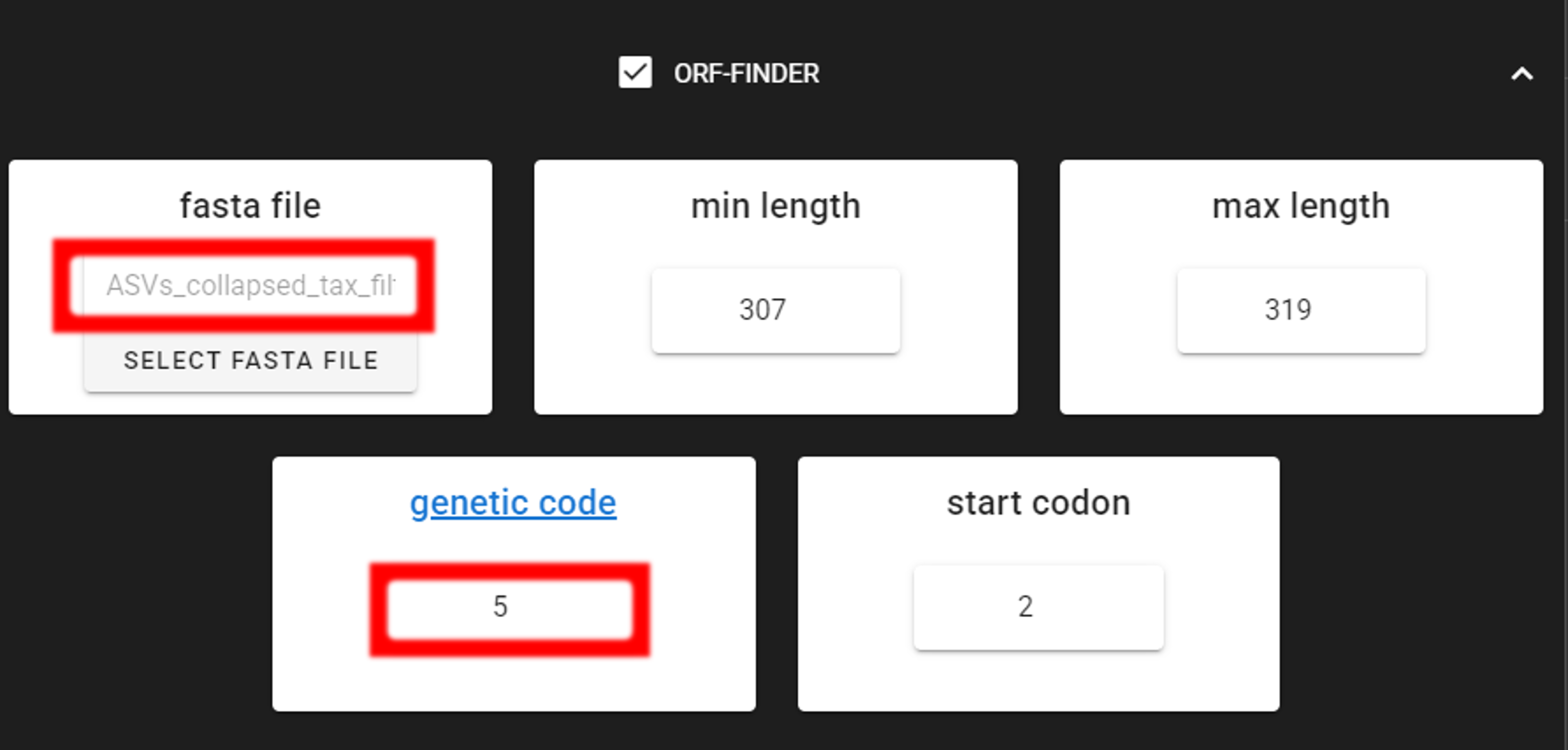
Here, we use ORFfinder.

Here, input data is only fasta file. We are selecting out filtered fasta file ASVs_collapsed_tax_filt.fasta. As we are interesed in “The Invertebrate Mitochondrial Code”, we as specifying 5 in the genetic code setting (in PipeCraft, click on the genetic code setting to see the available genetic codes). The min length and max length settings were already set in the CURATE ASV TABLE step, so here, those setting to not have an effect unless we narrow down the accepdable length range.

Double-check the selected working directory (the outputs will be written there) by holding the mouse cursor over the SELECT WORKDIR button [re-select if needed].

Press “START” to start the ORFfinder process.

---

Output files:
*_ORFs.fasta	fasta file of filtered ASVs
*_ORFs.list.txt	list of of filtered ASVs
*_notORFs.fasta	fasta file of ASVs that did not pass ORF-finder
*_notORFs.list.txt	list of ASVs that did not pass ORF-finder

This process filters only the fasta file and as a main output it creates a a list of ASVs that passed and did not pass the genetic code translation.

In this example dataset, ORFfinder identidied 1 ASV that did not pass the genetic code translation. Let’s discard this ASV from the dataset.

Below, you can find a R script to clean also taxonomy and ASV tables.

Remove NUMTs from taxonomy and ASV tables based on ORFfinder output

#!/usr/bin/env Rscript
### Filter dataset based on ORF-finder results to exclude putative NUMTs

# Specify input files
discard_file = "ASVs_collapsed_tax_filt.notORFs.list.txt"
fasta_file = "ASVs_collapsed_tax_filt.fasta"
ASV_table_file = "ASVs_table_collapsed_tax_filt.txt"
taxonomy_file = "taxonomy.sintax.filt.txt"
#--------------------------------------#
library(seqinr)

# Read the list of ASVs that should be discarded based on ORFfinder output
discard = read.table(discard_file, header = FALSE)
# Read the fasta file
fasta = read.fasta(fasta_file)
n_input = length(fasta)
# Read the ASV table
ASV_table = read.table(ASV_table_file, header = TRUE)
# Read the taxonomy file
taxonomy = read.table(taxonomy_file, header = TRUE)
### Remove ASVs from fasta file
fasta = fasta[!names(fasta) %in% discard$V1]

# Remove ASVs from ASV table
ASV_table = ASV_table[!ASV_table$ASV %in% discard$V1, ]

# Remove ASVs from taxonomy file
taxonomy = taxonomy[!taxonomy$ASV %in% discard$V1, ]

# Summary
cat("Number of input ASVs:", n_input, "\n")
cat("Number of ASVs discarded:", nrow(discard), "\n")
cat("Number of ASVs left:", length(fasta), "\n")

# Create output folder
outdir <- "ORF_filtered"
if (!dir.exists(outdir)) {
  dir.create(outdir)
}

# Output names: input basename with "_ORFs" before extension
add_ORFs <- function(f) {
  paste0(tools::file_path_sans_ext(basename(f)), "_ORFs.", tools::file_ext(f))
}

# Write outputs
write.fasta(fasta, names(fasta), nbchar = 999,
            file.path(outdir, add_ORFs(fasta_file)))
write.table(ASV_table, file.path(outdir, add_ORFs(ASV_table_file)),
            sep = "\t", quote = FALSE, row.names = FALSE)
write.table(taxonomy, file.path(outdir, add_ORFs(taxonomy_file)),
            sep = "\t", quote = FALSE, row.names = FALSE)

Output files

• ORF_filtered directory:

  • ASVs_collapsed_tax_filt_ORFs.fasta: fasta file of filtered ASVs

  • ASVs_table_collapsed_tax_filt_ORFs.txt: filtered ASV table

  • taxonomy.sintax.filt_ORFs.txt: filtered taxonomy table

Proceed with any relevant statistical analyses using these filtered files if you are interesed in ASV-level analyses, or proceed with clustering ASVs into OTUs (see below).

---

Cluster ASVs into OTUs

If the aim is not to do the haplotype-level analyses, then ASVs can be clustered into OTUs (PipeCraft uses vsearch for this). The ASVs approach may not accurately reflect species composition in the community of as COI gene has highly variable levels of intraspecific polymorphism. Thus, one species may be represented by many ASVs, whereas other species may be represented by very few ASVs.

Here, we are clustering ASVs to OTUs (using vsearch) via QuickTools panel (on the right ribbon).

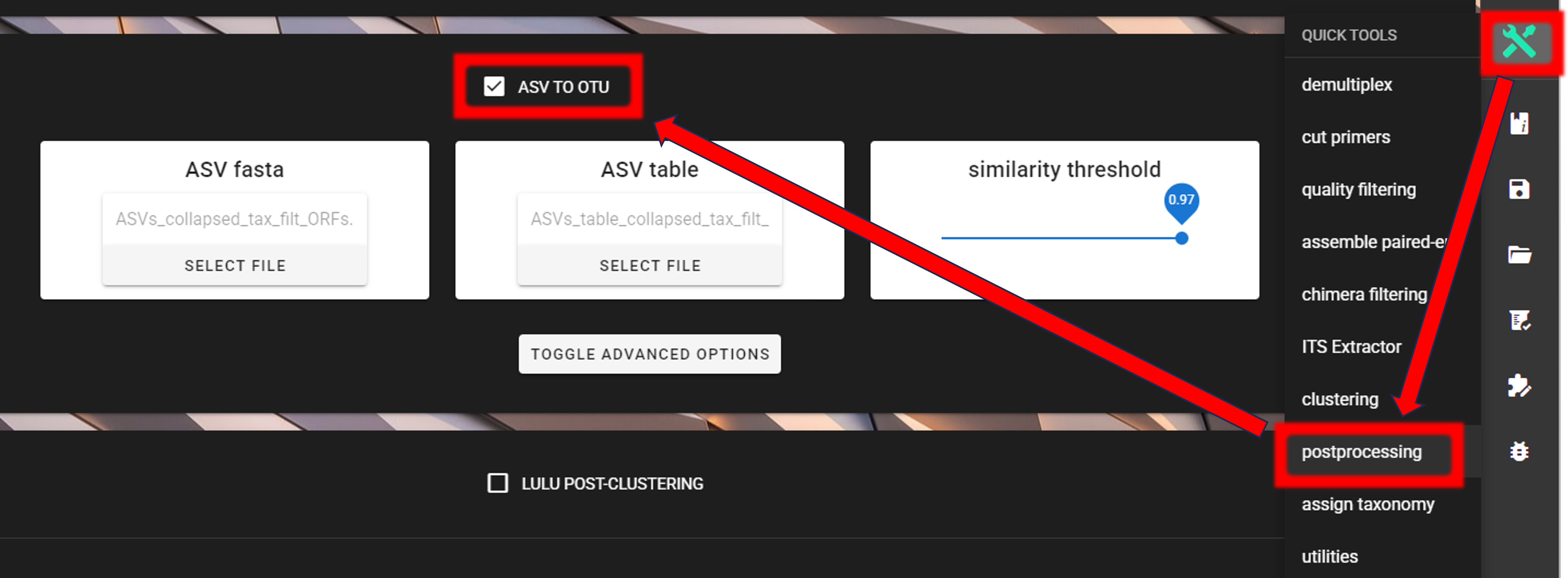
Input data are files in the ORF_filtered directory:

• ASVs_collapsed_tax_filt_ORFs.fasta

• ASVs_table_collapsed_tax_filt_ORFs.txt

As a similarity threshold we are using the commonly used 97% (0.97, default setting).

Note

2nd column of the input ASV table must be ‘Sequences’ (1st column is ASV IDs; this is the default PipeCraft2 output table, so you don’t need to worry about this if you have followed this pipeline). For clustering, the ASV size annotation is obtained from the ASV table.

If the ASV table does not contain ‘Sequence’ column, then add those with QuickTools -> Utilities -> Add sequences to table see here.

Specify ORF_filtered directory as a working directory via SELECT WORKDIR button and press “START” to start the process.

---

Outputs in ASVs2OTUs_out directory:
OTUs.fasta	FASTA formated representative OTU sequences
OTU_table.txt	OTU table (tab delimited file)
OTUs.uc	uclust-like formatted clustering results

Herein, clustering formed 17 OTUs from 19 ASVs (with 97% similarity threshold).

As we performed taxonomy annotation to ASVs, we can now match the taxonomy to the OTUs.

Get taxonomy for OTUs based on ASVs taxonomy

#!/usr/bin/env Rscript
### Get taxonomy for OTUs based on ASVs taxonomy

# Specify input files
# Working directory is "ASVs2OTUs_out"
ASV_taxonomy_file = "../taxonomy.sintax.filt_ORFs.txt"
OTU_fasta_file = "OTUs.fasta"
#--------------------------------------#
library(seqinr)

# Read the ASV taxonomy file
ASV_taxonomy = read.table(ASV_taxonomy_file, header = TRUE)
# Read the OTU fasta file
OTU_fasta = read.fasta(OTU_fasta_file)
# Get the taxonomy for each OTU
OTU_taxonomy = ASV_taxonomy[ASV_taxonomy$ASV %in% names(OTU_fasta), ]

# Write the OTU taxonomy file
write.table(OTU_taxonomy, file = "taxonomy.OTUs.txt", sep = "\t",
            quote = FALSE, row.names = FALSE, col.names = TRUE)

OTU taxonomy file

• taxonomy.OTUs.txt

When now comparing the ASVs and OTUs taxonomy tables, we can see that the ASVs taxonomy table had 2 ASVs assigned to Euzetes globulus species, and 2 ASVs assigned to Holoparasitus calcaratus species, but those are now merged respectively into 1 OTU for each of these species (with 97% similarity threshold).

However, in the OTUs taxonomy table, we see that Lithobius curtipes and Adoristes ovatus are represented by 2 OTUs, respectively. Certanly, the barcoding gaps may vary between different specie, thus resulting in different OTUs for the same species when using single sequence similarity threshold. But let’s check if the post-clustering process will help to merge these OTUs with same species names (see below).

---

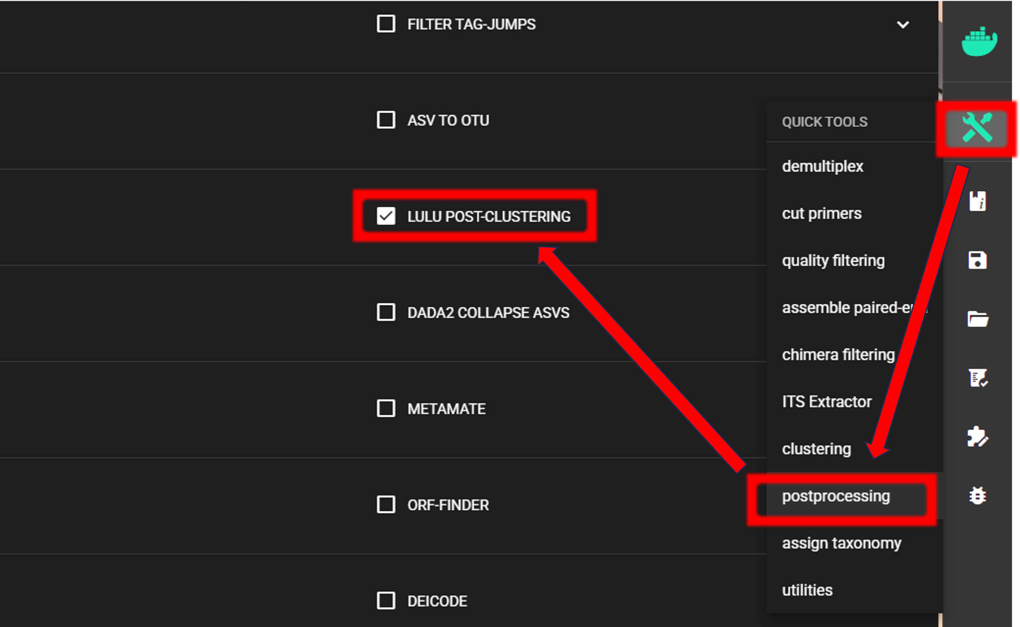
LULU post-clustering

Additionally, we can perform LULU post-clustering to merge co-occurring ‘daughter’ OTUs.

LULU description from the LULU repository: the purpose of LULU is to reduce the number of erroneous OTUs in OTU tables to achieve more realistic biodiversity metrics. By evaluating the co-occurence patterns of OTUs among samples LULU identifies OTUs that consistently satisfy some user selected criteria for being errors of more abundant OTUs and merges these. It has been shown that curation with LULU consistently result in more realistic diversity metrics.

Here, we are performing LULU post-clustering via QuickTools panel (on the right ribbon).

The input data are OTU_table.txt and OTUs.fasta files in the ASVs2OTUs_out directory. Here, we are using the default settings (which are suitable for most cases), but feel free to experiment with various settings to see the effect on the results.

To START

To START, specify working directory under SELECT WORKDIR (outputs will be written here), but the following requests about Sequence files extension and Sequencing read types do not matter here, just click ‘Confirm’.

Outputs in lulu_out directory:
OTU_table.lulu.txt	curated table in tab delimited txt format
OTUs.lulu.fasta	fasta file for the molecular units (OTUs or ASVs) in the curated table
match_list.lulu	match list file that was used by LULU to merge ‘daughter’ molecular units
discarded_units.lulu	molecular units (OTUs or ASVs) that were merged with other units based on specified thresholds

---

The input for LULU post-clustering had 17 OTUs, with double representation of Lithobius_curtipes and Adoristes_ovatus OTUs:

OTU	sample1_COI	sample2_COI	sample3_COI
Adoristes_ovatus Adoristes_ovatus Entomobrya_sp Euzetes_globulus Fridericia_eiseni Holoparasitus_calcaratus Lithobius_curtipes Lithobius_curtipes Orchesella_flavescens Pergalumna_nervosa Tomocerus_sp Trachytes_aegrota unclassified_Arthropoda_sp unclassified_Arthropoda_sp unclassified_Arthropoda_sp unclassified_Arthropoda_sp unclassified_Metazoa_sp	0 0 0 0 215 0 15 583 0 0 0 0 0 0 0 0 0	342 0 0 179 0 38 0 0 0 45 0 7 75 81 0 0 0	0 3 25 0 0 7 0 0 10 0 35 0 0 0 39 682 2

After LULU post-clustering, LULU merged 2 Lithobius_curtipes OTUs into a single Lithobius_curtipes OTU. But Adoristes ovatus remains represented as 2 OTUs.

OTU	sample1_COI	sample2_COI	sample3_COI
Adoristes_ovatus Adoristes_ovatus Entomobrya_sp Euzetes_globulus Fridericia_eiseni Holoparasitus_calcaratus Lithobius_curtipes Orchesella_flavescens Pergalumna_nervosa Tomocerus_sp Trachytes_aegrota unclassified_Arthropoda_sp unclassified_Arthropoda_sp unclassified_Arthropoda_sp unclassified_Arthropoda_sp unclassified_Metazoa_sp	0 0 0 0 215 0 598 0 0 0 0 0 0 0 0 0	342 0 0 179 0 38 0 0 45 0 7 75 81 0 0 0	0 3 25 0 0 7 0 10 0 35 0 0 0 39 682 2

In addition to sequence similarity, LULU post-clustering merges OTUs based on co-occurrence patterns, and as Adoristes ovatus OTUs are not co-occurring in the same samples, LULU did not merge them. On the other hand, Lithobius curtipes OTUs were both in sample1_COI, thus were merged into single Lithobius curtipes OTU by summing up the abundances of the two OTUs.

The last step

The last step here is to get matching taxonomy table for the LULU-curated OTUs.

Get final OTUs taxonomy table based on LULU results

#!/usr/bin/env Rscript
### Get final OTUs taxonomy

# Specify input files
OTUs_taxonomy_file = "taxonomy.OTUs.txt" # OTUs taxonomy table
OTU_fasta_file = "OTUs.lulu.fasta"       # LULU-curated OTUs fasta file
#--------------------------------------#
library(seqinr)

# Read the ASV taxonomy file
OTUs_taxonomy = read.table(OTUs_taxonomy_file, header = TRUE)
# Read the OTU fasta file
OTU_fasta = read.fasta(OTU_fasta_file)
# Get the taxonomy for each OTU
OTU_taxonomy = OTUs_taxonomy[OTUs_taxonomy$ASV %in% names(OTU_fasta), ]

# Write the OTU taxonomy file
write.table(OTU_taxonomy, file = "taxonomy.OTUs.lulu.txt",
            sep = "\t", quote = FALSE, row.names = FALSE)

Final curated OTU files

Now, final curated files are:

• taxonomy.OTUs.lulu.txt

• OTUs.lulu.fasta

• OTU_table.lulu.txt

Proceed with any relevant statistical analyses using the curated files.