vsearch OTUs pipeline, ITS2

This example data analyses follows vsearch OTUs workflow as implemented in PipeCraft2’s pre-compiled pipelines panel.

Download example data set here (15.1 Mb) and unzip it.

This is ITS2 Illumina MiSeq dataset.

For this example, we are using EUKARYOME database in the taxonomy annotation process (BLAST). Download the General_EUK_ITS file from here and unzip it (note: use 7-Zip software for unzipping files in Windows).

---

Starting point

This example dataset consists of ITS2 rRNA gene amplicon sequences; targeting fungi:

• paired-end Illumina MiSeq data;

• demultiplexed set (per-sample fastq files);

• primers are not removed;

• sequences in this set are 5’-3’ oriented.

when working with your own data …

… then please check that the paired-end data file names contain R1 and R2 strings (not just _1 and _2), so that PipeCraft can correctly identify the paired-end reads.

Example:

sample1_R1.fastq.gz

sample1_R2.fastq.gz

---

To select vsearch OTUs pipeline, press

SELECT PIPELINE –> vsearch OTUs.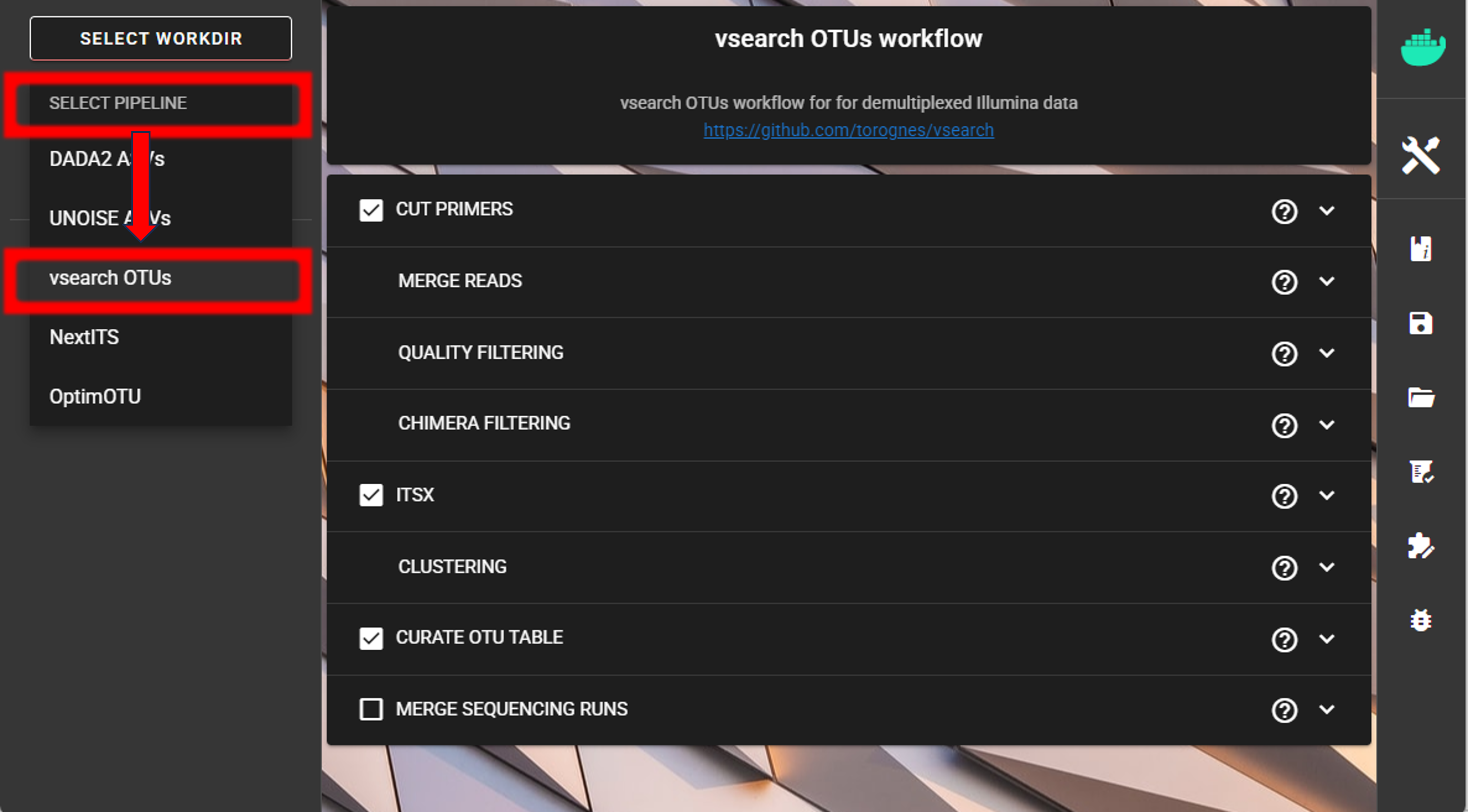

To select input data, press SELECT WORKDIR

and specify

sequence files extension as *.fastq.gz;

sequencing read types as paired-end.

---

Cut primers

The example dataset contains primer sequences. Generally, we need to remove these to proceed the analyses only with the variable metabarcode of interest. If there are some additional sequence fragments, from eg. sequencing adapters or poly-G tails, then clipping the primers will remove those fragments as well.

Tick the box for CUT PRIMERS and specify forward and reverse primers. For the example data, the forward primer is GTGARTCATCGAATCTTTG (fITS7) and reverse primer is TCCTCCGCTTATTGATATGC (ITS4).

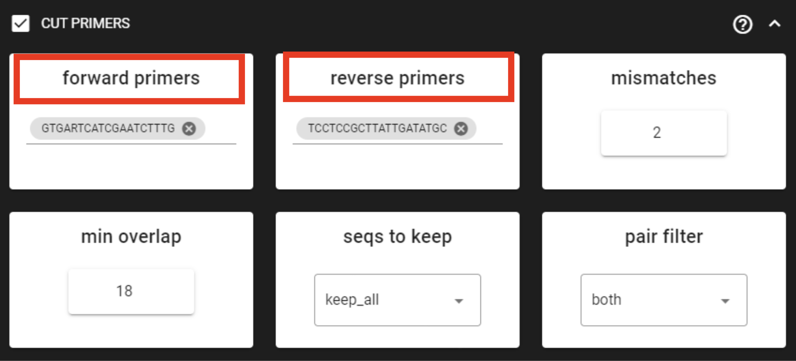
Forward primer has 19 bp and reverse 20 bp - to keep a bit of flexibility in the primer search, we are requesting the min overlap of 18 bp and are allowing maximum of 2 mismatches . Note that too low min overlap may lead to random matches. Check other CUT PRIMER options here.

Note

You may specify add up to 13 primer pairs.

A consideration when working with ITS sequences and plan to use ITS Extractor

Since fITS7 and ITS4 primer binding sites are >50 bp from ITS2 region from the 5.8S side and >40 bp from the 28S side, we can clip the primers in order to safely use ITS Extractor to remove the flanking regions from ITS2 reads.

However, when the primer binding sites are very close to the ITS region (< 25 bp), then you may want to keep the primers for better detection of the 18S, 5.8S and 28S regions.

---

Quality filtering

Quality filtering removes sequences, which do not meet the threshold for the allowed maximum number of expected errors (maxee; sum of per-base error probabilities derived from Phred scores).

If the quality profile of the sequences are low at the beginning or at the end, then applying trunc length, strip_left and strip_right settings may be helpful to remove low-quality ends/starts of reads before filtering (maxee filtering is applied to the truncated reads). See remove low-quality ends/starts of reads section.

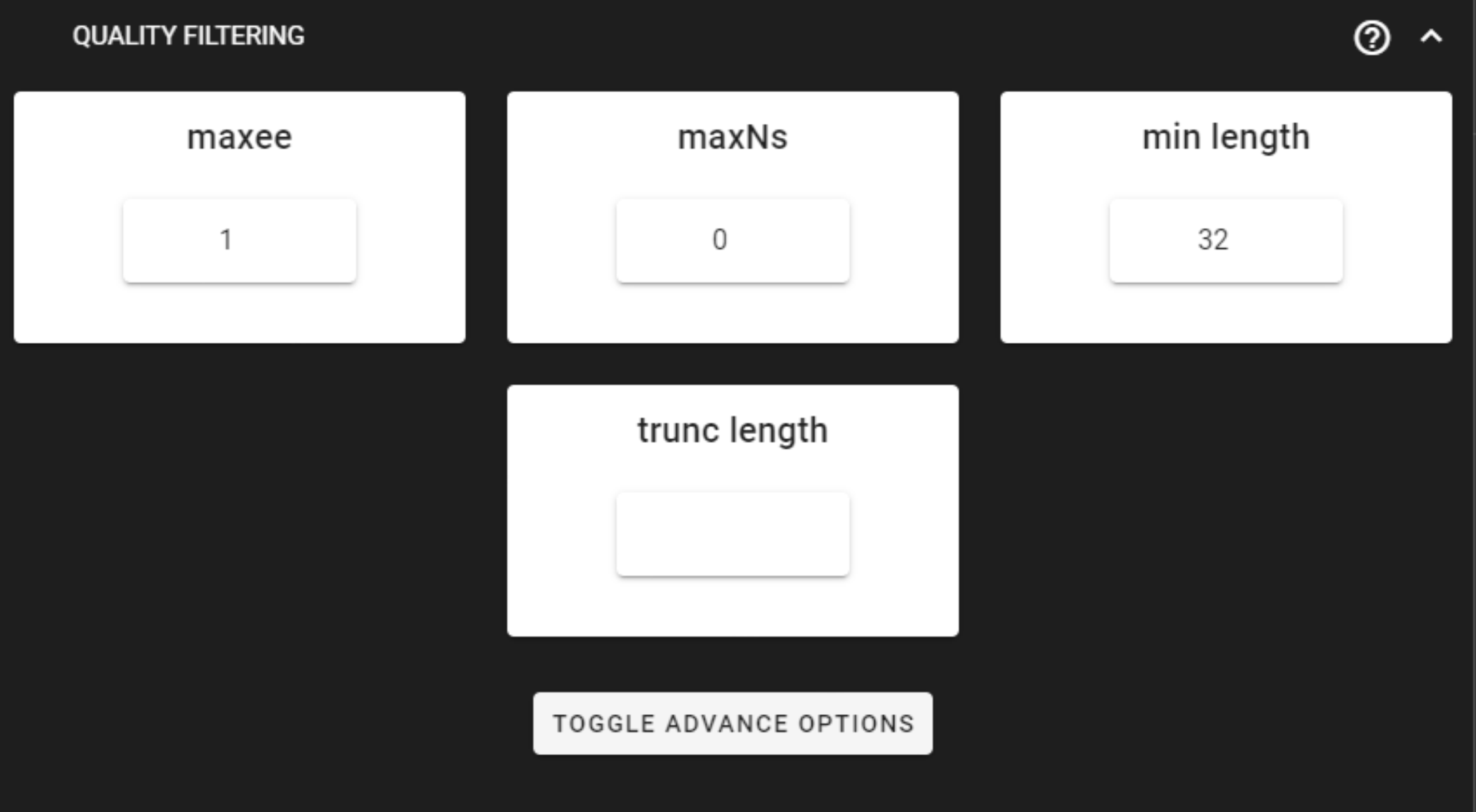
Here, we can leave settings as DEFAULT. Check the settings here.

Output directory qualFiltered_out
*.fastq	quality filtered sequences per sample in FASTQ format
seq_count_summary.txt	summary of sequence counts per sample

---

Merge paired-end reads

This step assembles/merges the paired-end read mates. Click on MERGE READS to expand the panel.

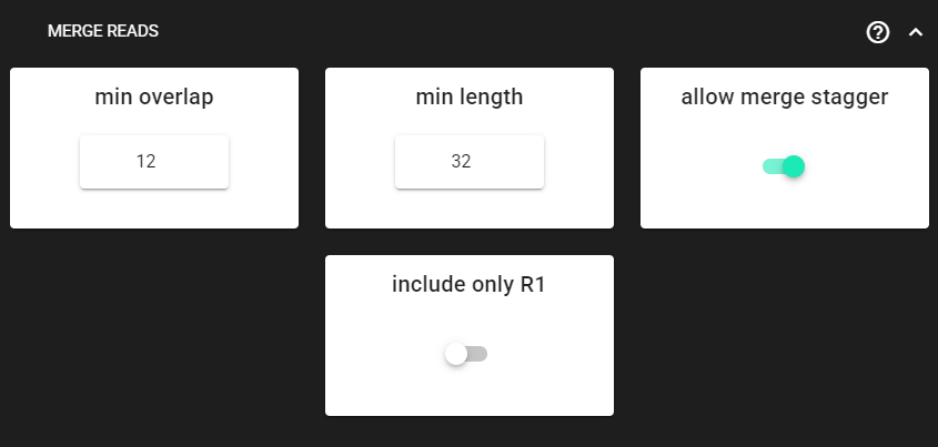
Here, we are using the DEFAULT settings, which are fine in most cases. Check other MERGE PAIRS options here.

Output directory assembled_out
*.fastq	merged per sample FASTQ files
seq_count_summary.txt	summary of sequence counts per sample

---

Chimera filtering

This step performs chimera filtering according to uchime algoritm, and optionally uchime_ref (reference based) algorithm.

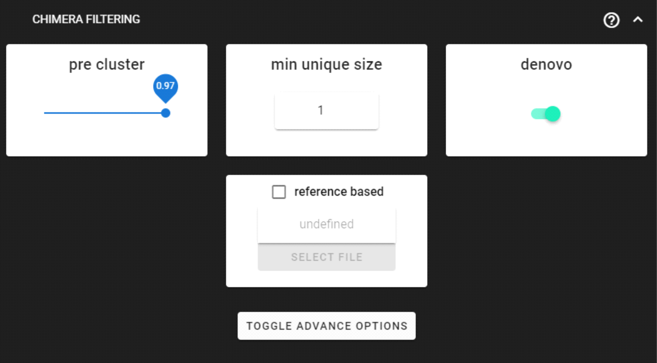
Here, we are using the DEFAULT settings. Chimera filtering settings here.

when working with your own ITS data …

… then UNITE database may used as a reference for the additional ‘reference based’ chimera filtering process. When both, denovo and reference based methods, are selected, then denovo process will be performed first, and uchime_ref if applied upon uchime_denovo results.

Download UNITE ref databse for chimera filtering here (select ‘UCHIME/USEARCH/UTAX/SINTAX reference datasets’).

Output directory chimera_Filtered_out
*.fasta	chimera filtered sequences per sample in FASTA format
seq_count_summary.txt	summary of sequence counts per sample
chimeras/*.fasta	discarded sequences per sample during chimera filtering

---

Extract ITS2

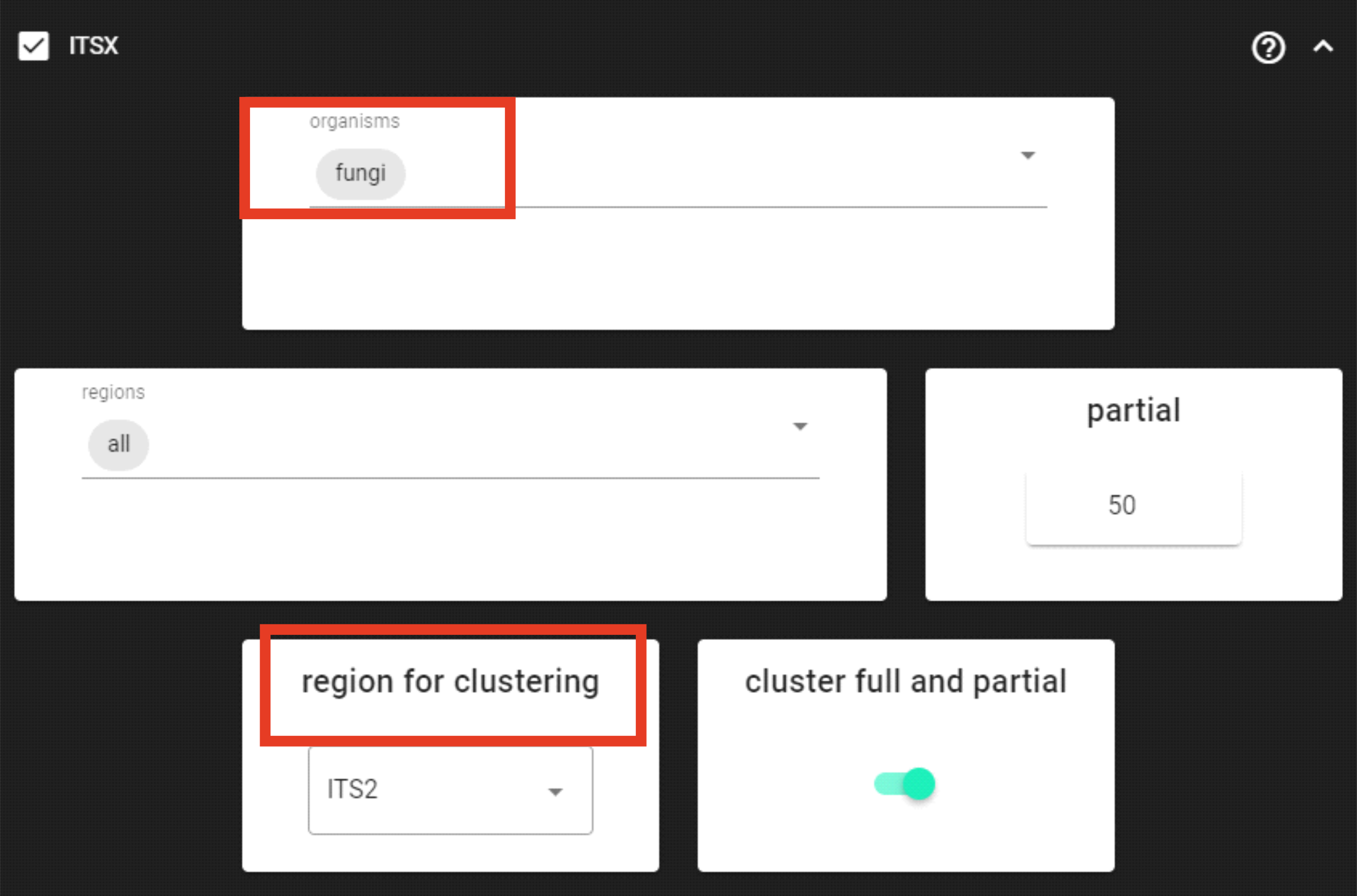
Here, in this example dataset, we are working with ITS2 amplicons, and we want to remove the conservative flanking regions (where the primer binding sites are located) that are affecting the clustering thresholds. For that, we are using ITSx.

Since we are working with ITS2 amplicons and are interesed only in fungi, we can limit the organisms to only fungi and keep the region for clusering as ITS2. Since universal ITS2 primers amplify also other eukaryotes besides fungi, this step helps also to discard off-target sequences when limiting the organisms to only fungi. However, note that this increase in specificity may lead to some decrease in sensitivity; i.e., discarding some Fungal OTUs. For real-world applications, you may set organism to “all”, and discard off-target OTUs after the taxonomy assignment step (see below).

when working with your own ITS data …

… then double-check the region for clusering setting and edit according to your working amplicon (ITS1/ITS2,full-ITS). Since, ITSx outputs multiple directories for corresponding ITS regions, we need to specify the region for clusering accordingly so that PipeCraft can proceed with clustering the corresponding ITS region.

If you are working with only 5’-3’ oriented amplicons, then turn off complement setting under TOGGLE ADVANCE OPTIONS to skip the reverse complementary search; and possibly add more cores to speed things up (see here).

The partial setting is set to 50, which means that if at least one of the 5.8S or 28S motif is found in the sequence and that sequence is at least 50 bp long (after cutting the motif), then it will be classified as partial ITS2 sequence and outputted in the ITS2/full_and_partial directory.

cluster full and partial is ON, which means that in the following process (clustering), PipeCraft is clustering sequences in the ITS2/full_and_partial directory. In most cases, this is fine as the partial ITS2 sequences are clustered together with the full ITS2 sequences (if they fall into the same similarity threshold). But this behaviour can be turned off by turning off the cluster full and partial setting.

Note

For better detection of the 18S, 5.8S and/or 28S regions by ITSx, you may not want to CUT PRIMERS in your own dataset. With this example dataset, ITSx works fine even when primers were clipped.

Output directory ITSx_out
ITS2/*.fasta	ITS2 sequences (without flanking gene fragments) per sample
ITS2/full_and_partial/*.fasta	full, but also partial ITS2 sequences per sample
seq_count_summary.txt	summary of sequence counts per sample

---

Clustering

The clustering process collapses sequences that fall into the same similarity threshold using vsearch clustering algorithms. Check vsearch clustering settings here to see the supported methods.

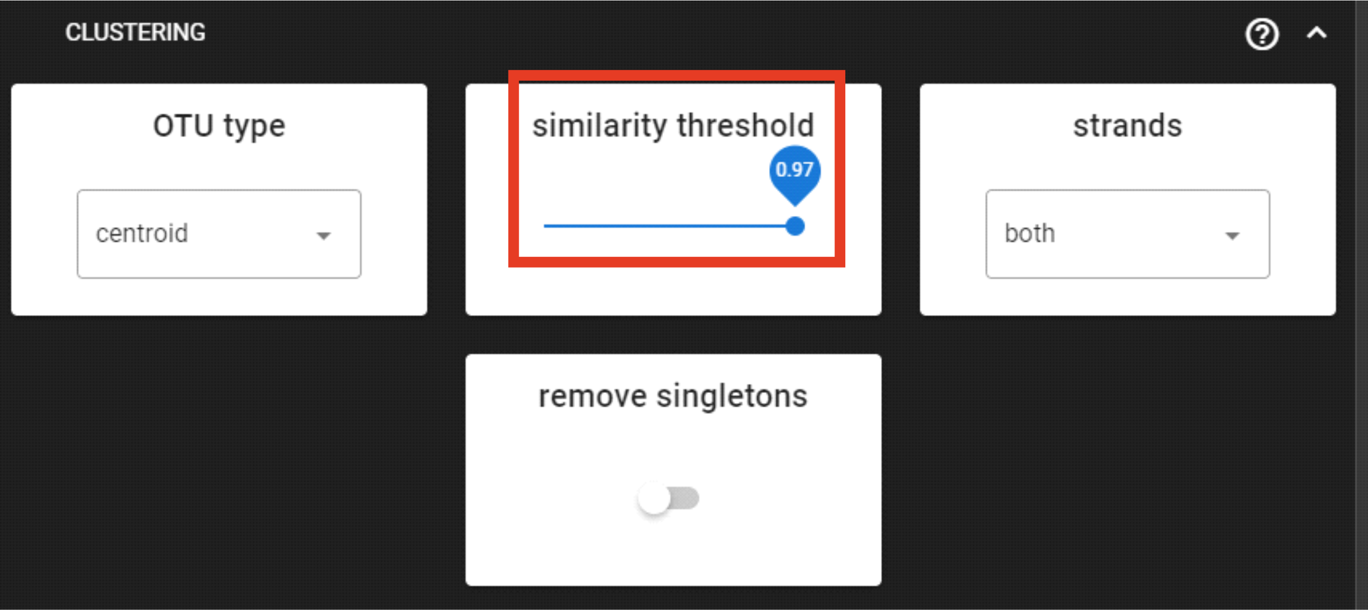
Here, we are applying DEFAULT settings by clustering sequenes with 97% similarity threshold. Here, however, the strands could be set as “plus” (for the process to be a bit faster), since our sequences are 5’-3’ oriented (keep it “both” when sequences are mixed orientations in the dataset).

Output directory clustering_out
OTU_table.txt	OTU-by-sample table
OTUs.fasta	corresponding FASTA formated OTU sequences
OTUs.uc	clustering results mapping file

---

Curate ASV table

This process first removes putative tag jumps and then filters out OTUs whose sequences are shorter/longer than specified length (in base pairs).

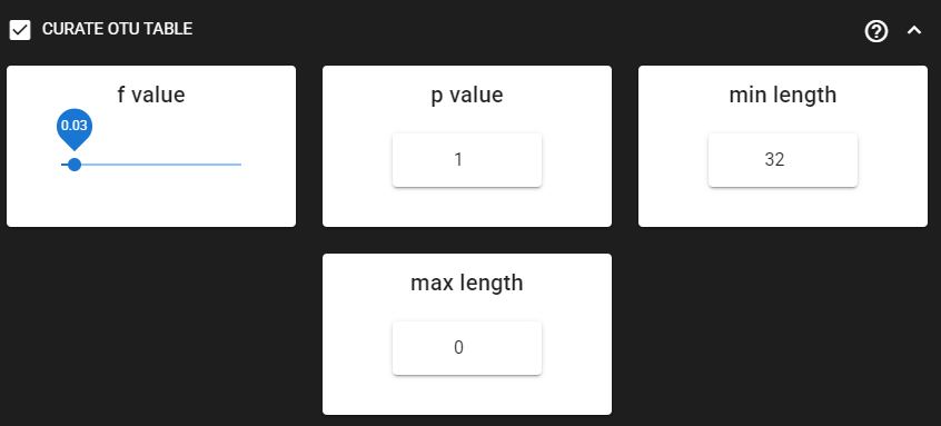
Here, we are enabling this process by checking the box for CURATE OTU TABLE in the workflow panel.

The f_value and p_value settings are used to filter out putative tag jumps (using UNCROSS2 algorithm). Generally, we recommend to use p_value of 1 (default), and f_value of 0.03 when using combinational indexing strategy; f_value of 0.05 when using single-indexes, and f_value of 0.01 when using unique dual-indexes.

Since the ITS2 sequences are highly variable among Fungi, we are keeping the max length as 32 (bp) and max length as 0 (meaning no filtering by maximum sequence length).

Output directory	clustering_out/curated
OTU_table_TagJumpFilt.txt	only tag-jump filtered OTU-by-sample table
OTUs.fasta	corresponding OTU sequences
TagJump_stats.txt	summary of tag-jump filtering results

Note

OTU_table_TagJumpFilt.txt is outputted even when there are no tag-jump events detected. In this case, OTU_table_TagJumpFilt.txt is the same as OTU_table.txt in the clustering_out directory.

---

Save workflow

Once we have decided about the settings in our workflow, we can save the configuration file by pressing save workflow button on the right-ribbon

If you forget the save, then no worries, a pipecraft2_last_run_configuration.json file will be generated for you upon starting the workflow. As the file name says, it is the workflow configuration file for your last PipeCraft run in this working directory. If the file name (pipecraft2_last_run_configuration.json) is not changed, then the file is overwritten with the new configuration if running a new job in the same working directory.

This JSON file can be loaded into PipeCraft2 to automatically configure your next runs exactly the same way.

Note

‘Assign taxonomy’ is not the part of the full per-defined pipeline. This step can be selected and run via QuickTools panel. See below.

---

Start the workflow

Press START on the left ribbon to start the analyses.

when running the module for the first time …

… a docker image will be first pulled to start the process.

For example:

When you need to STOP the workflow, press STOP button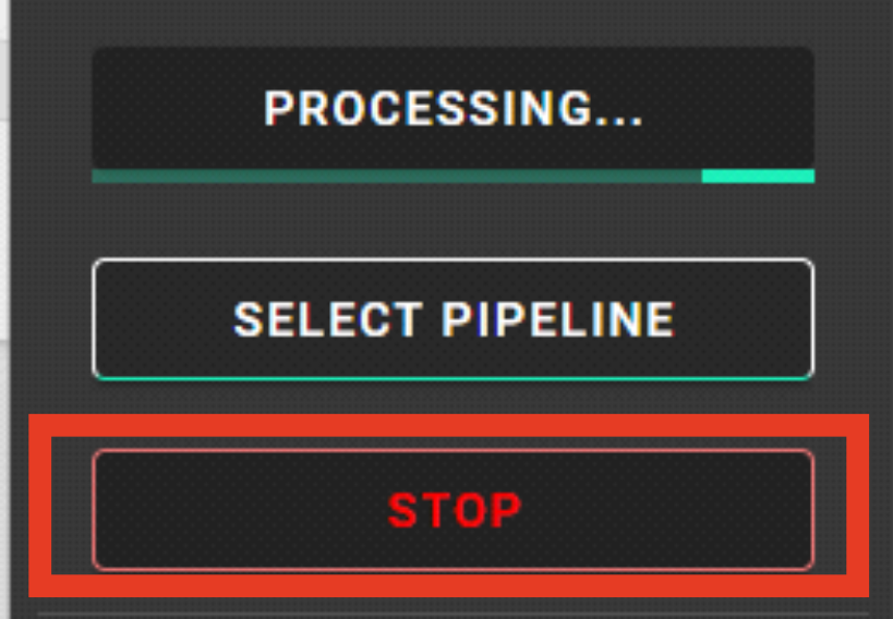

When the workflow has completed …

… a message window will be displayed.

---

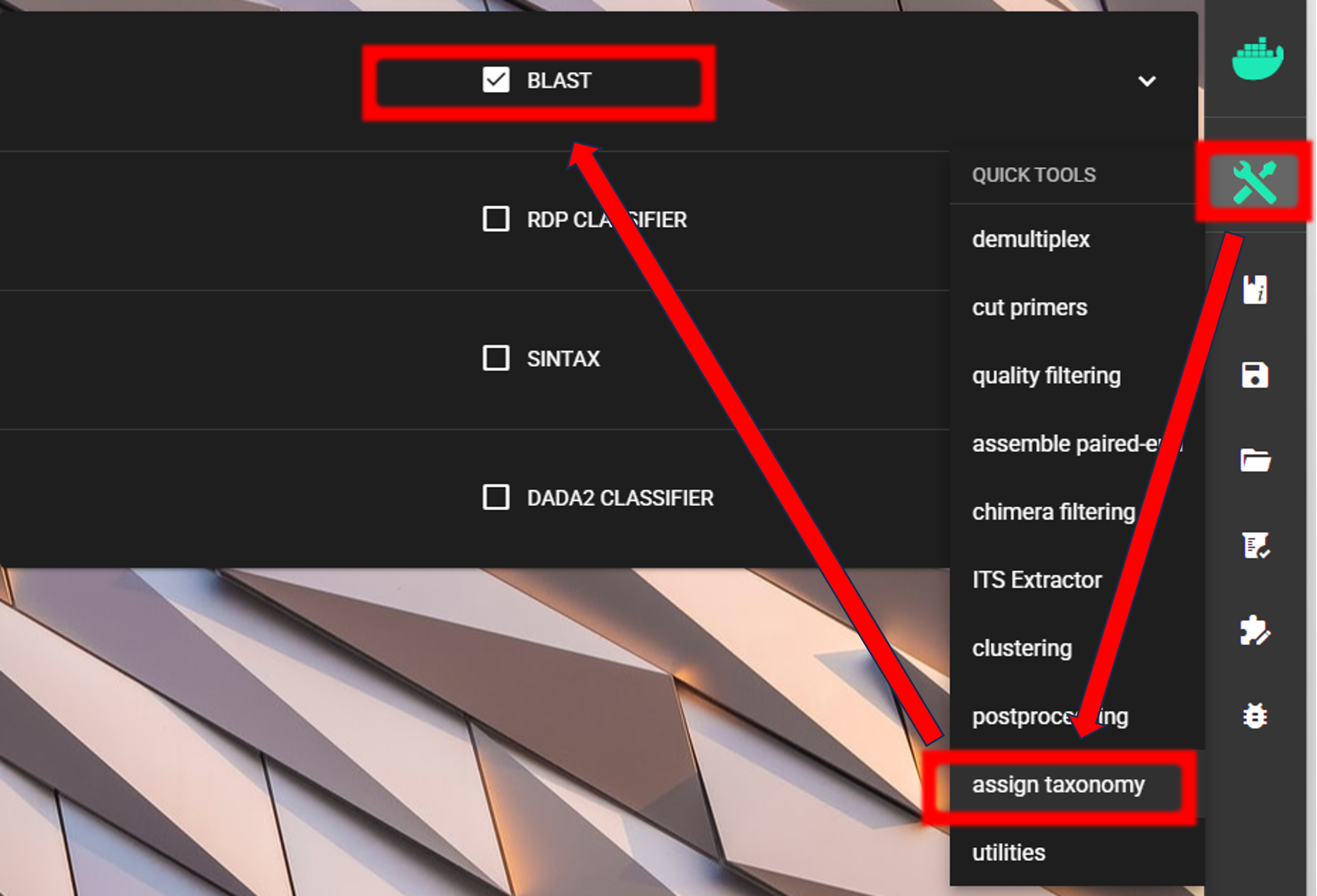
Assign taxonomy

Assign taxonomy is not the part of the full per-defined pipeline, but can be run as a separate step in QuickTools.

Here, we are using BLAST. See other assign taxonomy options here.

We need to specify the location of the reference DATABASE for the taxonomic classification of our OTUs. For this example, we are using EUKARYOME database, which is a comprehensive database of eukaryotic ITS sequences; thus containing also other eukaryotic sequences besides Fungi. “Outgroups” are important in the reference database in order not to overclassify non-Fungal sequences as Fungi. Download the General_EUK_ITS file from here and unzip it (note: use 7-Zip software for unzipping files in Windows).

See other databases available for taxonomy annotation here.

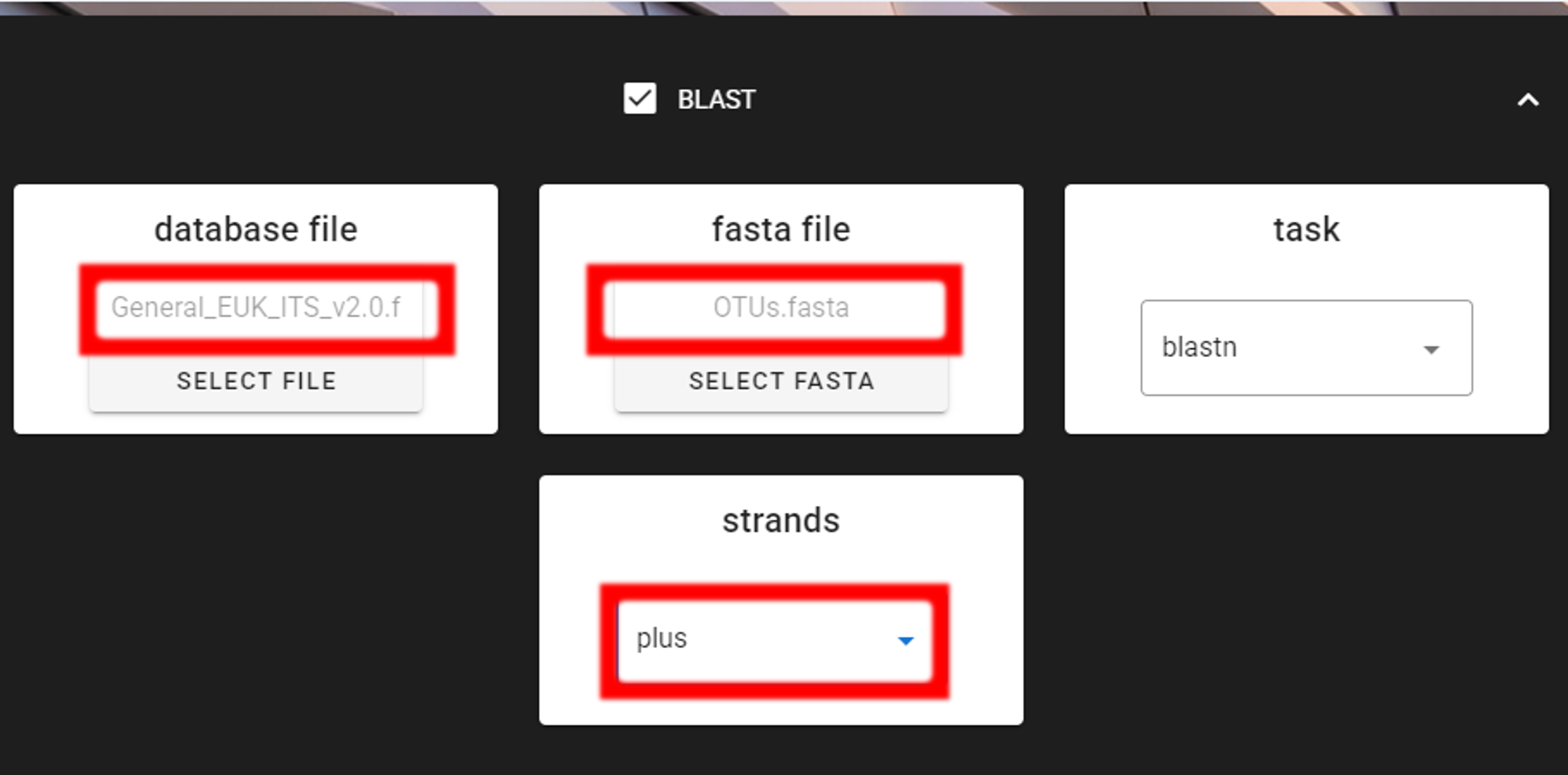
Specify the location of your downloaded database and also the fasta file with OTUs (fasta file) to be classified. Herein, we use OTUs.fasta file in the clustering_out/curated directory (since we applied also CURATE OTU TABLE process).

Important

Make sure you do not have any other BLAST database files is the same directory as the database you are using. That is, use dedicated directory for the BLAST database.

Here, we have 5’-3’ oriented OTUs, so let’s change the strands setting to “plus” (only forward strand search is performed) to speed up BLAST search.

Here, the task is blastn, which is suitable for sequences with moderate to distant similarity and is therefore preferred when comparing sequences across taxa or when sequence divergence is expected. The alternative option is megablast, which is optimized for the rapid alignment of highly similar nucleotide sequences and is typically used when sequences are expected to be nearly identical (e.g. within species); megablast is substantially faster than blastn, but less sensitive to divergent matches. Note that the sensitivity settings can be adjusted under TOGGLE ADVANCE OPTIONS panel.

To START

To START, specify working directory under SELECT WORKDIR (outputs will be written here), but the following requests about Sequence files extension and Sequencing read types do not matter here, just click ‘Confirm’.

Output directory	output_icon| taxonomy_out.blast
BLAST_1st_best_hit.txt	BLAST results for the 1st best hit in the used database.
BLAST_10_best_hits.txt	BLAST results for the 10 best hits in the used database.

---

Examine the outputs

Several process-specific output folders are generated

primersCut_out	paired-end fastq files per sample where primers have been cut
assembled_out	merged fastq files per sample
qualFiltered_out	quality filtered fastq files per sample
chimeraFiltered_out	chimera filtered fasta files per sample
ITSx_out	ITS2 sequences per sample without flanking gene fragments
clustering_out	OTU table, and OTU sequences files
taxonomy_out.blast	BLAST taxonomy assignment results

Each folder (except clustering_out and taxonomy_out) contain summary of the sequence counts (seq_count_summary.txt). Examine those to track the read counts throughout the pipeline.

For example, from the seq_count_summary.txt file in qualFiltered_out we see that first two samples did not contains much of bad quality sequences, while most of the sequences were discarded from the last three samples (note that this is an example dataset, with intentionally lower quality sequences in the last three samples).

File	Reads_in	Reads_out
sample1.fastq	22736	22661
sample2.fastq	13715	13393
sample3.fastq	11613	392
sample4.fastq	11456	23
sample5.fastq	9408	17

---

Final outputs of the pipeline

Here, we applied also “CURATE OTU TABLE” process. Therefore, our final outputs of the pipeline are in the clustering_out/curated directory, which contans:

OTU_table_TagJumpFilt.txt	tag-jump filtered OTU-by-sample table
OTUs.fasta	corresponding OTU Sequences with OTU_table_TagJumpFilt.txt table
TagJump_stats.txt	summary of tag-jump filtering results

If we see the OTU_table_TagJumpFilt_lenFilt.txt in the clustering_out/curated directory, then this means that some OTUs were discarded because of the length filtering.

Let’s check the README.txt file: there we can read that input OTU table for curation (clustering_out/OTU_table.txt) had 20 OTUs and the output OTU table (clustering_out/curated/OTU_table_TagJumpFilt_lenFilt.txt) has also 20 OTUs, since we did not apply length filtering, but only tag-jump filtering which does not affect the number of OTUs.

OTU_table_TagJumpFilt.txt represents the OTU table after the tag-jump filtering, where the 1st column represents OTU identifiers (sha1 encoded), 2nd column is the sequence of an OTU, and all the following columns represent number of sequences in the corresponding samples (sample name is taken from the file name). This is tab delimited text file.

OTU_table.txt; first 4 samples and 4 ASVs

OTU	Sequence	sample1ITS2full_and_partial	sample2ITS2full_and_partial	sample3ITS2full_and_partial
920bdde8…	AATCCT…	3814	4106	266
0ccd85db…	AATTCT…	3366	2101	0
80249b06…	AATCAT…	2868	1345	0
0e76c4ee…	ACAACC…	2052	736	0

Why our sample names have “ITS2full_and_partial” string attached??

Note that during the Extract ITS2 process the cluster full and partial was switched on and partial = 50. This means, that if at least one of the 5.8S or 28S motif is found in the sequence, and the sequence is at least 50 bp long (after cutting the motif), then the sequence will be passed into ITS2_full_and_partial output. And since the cluster full and partial was ON, the sample name is extended with “ITS2full_and_partial”.

We applied also tag-jump filtering process (via f_value and p_value settings). When checking the TagJump_stats.txt file in the clustering_out/curated directory, we see that based on our settings, 19 tag-jump events were detected which involved 143 reads. That is, there were 19 potential cases where an OTU may have been “leaked” from one sample to another. The number of OTUs are the same in clustering_out/OTU_table.txt and clustering_out/curated/OTU_table_TagJumpFilt.txt files, but clustering_out/curated/OTU_table_TagJumpFilt.txt file has 143 less reads than clustering_out/OTU_table.txt file as those were removed as putative tag-jumps.

So, for further processes, we use clustering_out/curated/OTU_table_TagJumpFilt.txt file, and clustering_out/curated/OTUs.fasta file.

---

Results from the taxonomy annotation process (BLAST) are located at the taxonomy_out.blast directory.

Output directory	output_icon| taxonomy_out.blast
BLAST_1st_best_hit.txt	BLAST results for the 1st best hit in the used database.
BLAST_10_best_hits.txt	BLAST results for the 10 best hits in the used database.

These files are “+”-delimited text files. Check the README.txt in the taxonomy_out.blast directory for more details about column headers.

Let’s examine the BLAST_1st_best_hit.txt file:

qseqid	query_seq	qseqid	1st_hit	qlen	slen	qstart	qend	sstart	send	evalue	length	nident	mismatch	gapopen	gaps	sstrand	qcovs	pident	sim_score	adj_qcov
02f4053… 0ccd85d… 0e76c4e…	TACTCTCA… AATTCTCA… ACAACCAG…	02f4053… 0ccd85d… 0e76c4e…	UDB025020;k__Fungi;p__Basidiomycota;c__Agaricomycetes;o__Sebacinales;f__Sebacinaceae;g__Sebacina;s__incrustans UDB016429;k__Fungi;p__Basidiomycota;c__Agaricomycetes;o__Atheliales;f__Atheliaceae;g__Athelia;s__bombacina UDB015480;k__Fungi;p__Ascomycota;c__Pezizomycetes;o__Pezizales;f__Pyronemataceae;g__Humaria;s__hemisphaerica	198 201 207	534 558 623	1 1 1	198 201 207	337 358 417	534 558 623	2.56E-97 6.13E-99 3.51E-102	198 201 207	198 201 207	0 0 0	0 0 0	0 0 0	plus plus plus	100 100 100	100 100 100	100 100 100	100 100 100

One of the most informative column is the sim_score column. This indicates the similarity of the OTU sequence to the target sequence in the reference database taking the query coverage into account. sim_score = similarity score of a hit taking the query coverage into account; calculated as (pident * (alignment length / qlen)). Therefore, it helps to identify hits with high identity% but low coverage to reference sequence (that is, only partial matches).

Important

If the OTU sequence gets a BLAST hit, and the 1st_hit column has taxonomy information down to species level, but the BLAST values are poor, then it is not appropriate to consider this OTU as assigned to this species. BLASTs results should be subjected to additional threshold filtering (see below).

The minimum similarity score for those OTUs in the example dataset is >99, with all hits to Fungi, so it is highly likely that all OTUs are Fungal OTUs, and here, we do not need to discard any off-target OTUs.

Below is the R-script for additional parsing of the BLAST results and discarding non-Fungal OTUs (if there are any). The script applies e-value and sim_score thresholds to parse the taxonomy information. Default threshold values are spcified according to Tedersoo et al. 2014.

This R-script works only for PipeCraft2 BLAST outputs with EUKARYOME database.

Parse BLAST_1st_hit results and discard non-target OTUs (if any)

#!/usr/bin/env Rscript
### Parse BLAST_1st_hit results and discard non-target OTUs (if any)

### Specify input file
 # BLAST 1st hit output from PipeCraft
blast_1st_hit_file = "BLAST_1st_best_hit.txt"

### Specify target group(s) (if any)
 # Target taxonomic group(s) to keep
target = c("Fungi")
 # Taxonomic level to filter on:
 #           Kingdom | Phylum | Class | Order | Family | Genus | Species
tax_level = "Kingdom"

### Specify sim_score thresholds for taxonomic levels
# Minimum sim_score required for reliable assignment at each level
sim_score_thresholds = list(
  Class = 75,
  Order = 80,
  Family = 85,
  Genus = 90,
  Species = 97
)

### Specify e-value thresholds
# e-value < e-50: reliable for kingdom assignment
# e-value > e-20: mark as "unknown"
evalue_reliable = 1e-50  # Reliable threshold for kingdom assignment
evalue_unknown = 1e-20   # Unknown threshold, mark OTU as "unknown"
#--------------------------------------#
#--------------------------------------#

# Load blast_1st_hit_file
blast_1st_hit = read.table("BLAST_1st_best_hit.txt",
                          header = TRUE, sep = "+", fill = TRUE)

###################################
### Parse 1st best hit taxonomy ###
###################################
### Parse semicolon-separated taxonomy
# Format: Accession;k__Kingdom;p__Phylum;
#           c__Class;o__Order;f__Family;g__Genus;s__Species
parse_taxonomy = function(taxonomy_string) {
  # Initialize result with NAs
  result = data.frame(
    Accession = NA, Kingdom = NA, Phylum = NA, Class = NA,
    Order = NA, Family = NA, Genus = NA, Species = NA,
    stringsAsFactors = FALSE
  )

  # Handle NA/empty cases
  if (is.na(taxonomy_string) ||
      taxonomy_string == "" ||
      taxonomy_string == "*") {
    return(result)
  }

  # Split by semicolon
  ranks = strsplit(taxonomy_string, ";")[[1]]

  # Extract accession number (first field)
  if (length(ranks) > 0) {
    result$Accession = ranks[1]
  }

  # Parse each rank (format: prefix__taxon_name)
  for (rank in ranks) {
    if (grepl("^k__", rank)) {
      # Kingdom
      result$Kingdom = sub("^k__", "", rank)
    } else if (grepl("^p__", rank)) {
      # Phylum
      result$Phylum = sub("^p__", "", rank)
    } else if (grepl("^c__", rank)) {
      # Class
      result$Class = sub("^c__", "", rank)
    } else if (grepl("^o__", rank)) {
      # Order
      result$Order = sub("^o__", "", rank)
    } else if (grepl("^f__", rank)) {
      # Family
      result$Family = sub("^f__", "", rank)
    } else if (grepl("^g__", rank)) {
      # Genus
      result$Genus = sub("^g__", "", rank)
    } else if (grepl("^s__", rank)) {
      # Species: combine with genus as Genus_species
      species_epithet = sub("^s__", "", rank)
      if (!is.na(result$Genus) && result$Genus != "") {
        result$Species = paste0(result$Genus, "_", species_epithet)
      } else {
        result$Species = species_epithet
      }
    }
  }

  return(result)
}

# Apply parsing function
taxonomy_parsed = do.call(rbind,
                          lapply(blast_1st_hit$X1st_hit, parse_taxonomy))

# Compile parsed 1st hit file
blast_taxonomy = cbind(
  qseqid = blast_1st_hit$qseqid,
  query_seq = blast_1st_hit$query_seq,
  taxonomy_parsed,
  qlen = blast_1st_hit$qlen,
  evalue = blast_1st_hit$evalue,
  nident = blast_1st_hit$nident,
  mismatch = blast_1st_hit$mismatch,
  qcovs = blast_1st_hit$qcovs,
  adj_qcov = blast_1st_hit$adj_qcov,
  pident = blast_1st_hit$pident,
  sim_score = blast_1st_hit$sim_score)

##############################################
### Apply e-value and sim_score thresholds ###
##############################################
# Mark as "unknown" if e-value > e-20
unknown_mask = blast_taxonomy$evalue > evalue_unknown
blast_taxonomy$Kingdom[unknown_mask] = "unknown"
blast_taxonomy$Phylum[unknown_mask] = NA
blast_taxonomy$Class[unknown_mask] = NA
blast_taxonomy$Order[unknown_mask] = NA
blast_taxonomy$Family[unknown_mask] = NA
blast_taxonomy$Genus[unknown_mask] = NA
blast_taxonomy$Species[unknown_mask] = NA

# Apply sim_score thresholds for valid hits (e-value < e-20)
valid_mask = blast_taxonomy$evalue < evalue_unknown

# Class threshold
class_below = valid_mask & (!is.na(blast_taxonomy$sim_score) &
                              blast_taxonomy$sim_score <
                              sim_score_thresholds$Class)
blast_taxonomy$Class[class_below] = NA
blast_taxonomy$Order[class_below] = NA
blast_taxonomy$Family[class_below] = NA
blast_taxonomy$Genus[class_below] = NA
blast_taxonomy$Species[class_below] = NA

# Order threshold
order_below = valid_mask & (!is.na(blast_taxonomy$sim_score) &
                              blast_taxonomy$sim_score <
                              sim_score_thresholds$Order) &
  !is.na(blast_taxonomy$Class)
blast_taxonomy$Order[order_below] = NA
blast_taxonomy$Family[order_below] = NA
blast_taxonomy$Genus[order_below] = NA
blast_taxonomy$Species[order_below] = NA

# Family threshold
family_below = valid_mask & (!is.na(blast_taxonomy$sim_score) &
                              blast_taxonomy$sim_score <
                              sim_score_thresholds$Family) &
  !is.na(blast_taxonomy$Order)
blast_taxonomy$Family[family_below] = NA
blast_taxonomy$Genus[family_below] = NA
blast_taxonomy$Species[family_below] = NA

# Genus threshold
genus_below = valid_mask & (!is.na(blast_taxonomy$sim_score) &
                              blast_taxonomy$sim_score <
                              sim_score_thresholds$Genus) &
  !is.na(blast_taxonomy$Family)
blast_taxonomy$Genus[genus_below] = NA
blast_taxonomy$Species[genus_below] = NA

# Species threshold
species_below = valid_mask & (!is.na(blast_taxonomy$sim_score) &
                                blast_taxonomy$sim_score <
                                sim_score_thresholds$Species) &
  !is.na(blast_taxonomy$Genus)
blast_taxonomy$Species[species_below] = NA

#######################################
### Filter to target group (if any) ###
#######################################
# Discard OTUs that are not classified as target at specified taxonomic level
if (length(target) > 0 && !all(is.na(target)) && target[1] != "") {
  if (tax_level %in% colnames(blast_taxonomy)) {
    n_before = nrow(blast_taxonomy)
    blast_taxonomy = blast_taxonomy[blast_taxonomy[[tax_level]] %in%
                                      target, , drop = FALSE]
    n_after = nrow(blast_taxonomy)
    n_excluded = n_before - n_after
    cat("\n Filtered to", tax_level, "level:",
        paste(target, collapse = ", "), "\n")
    cat(" Excluded", n_excluded, "OTUs not matching target.\n")
    cat(" Remaining OTUs:", n_after, "\n")
  } else {
    warning(paste("Column '", tax_level,
                  "' not found in taxonomy table; no filtering applied.",
                  sep = ""))
  }
}

# Write output
write.table(blast_taxonomy, file = "BLAST_1st_hit_parsed.txt",
            sep = "\t", quote = FALSE, row.names = FALSE)

---

Note

Alternatively, apply this script (Right-click → Save As) to generate the consensus taxonomy from the 10 best hits [method explanation is in the script].

Here, with this example dataset, we did not have any non-Fungal OTUs to be filtered out, but in case some OTUs were discarded from the BLAST results, then use the following R-script to filter the OTU table and fasta file accordingly.

Filter OTU table and fasta file based on taxonomy table (BLAST_1st_hit_parsed.txt)

#!/usr/bin/env Rscript
### Filter OTU table and fasta file based on taxonomy table (BLAST_1st_hit_parsed.txt)

### Specify input files
# OTU table
otu_table_file = "../OTU_table_TagJumpFilt.txt"
# OTU fasta file
otu_fasta_file = "../OTUs.fasta"
# BLAST_1st_hit_parsed.txt
blast_1st_hit_parsed_file = "BLAST_1st_hit_parsed.txt"
#--------------------------------------#
library(dplyr)
library(readr)
library(Biostrings)

# Load BLAST taxonomy file
blast_taxonomy = read.table(blast_1st_hit_parsed_file,
                            header = TRUE, sep = "\t",
                            stringsAsFactors = FALSE)

# Get list of OTU IDs from BLAST file
otu_ids_keep = unique(blast_taxonomy$qseqid)

# Load OTU table
otu_table = read.table(otu_table_file,
                      header = TRUE, sep = "\t",
                      stringsAsFactors = FALSE)

# Filter OTU table - keep only OTUs in BLAST file
otu_table_filtered = otu_table[otu_table[, 1] %in% otu_ids_keep, ]

# Write filtered OTU table
write.table(otu_table_filtered,
            file = "OTU_table_filtered.txt",
            sep = "\t", quote = FALSE, row.names = FALSE)

# Load OTU fasta file
otu_fasta = readDNAStringSet(otu_fasta_file)

# Extract OTU IDs from fasta names (assuming format is just OTU ID or OTU_ID;description)
otu_names = names(otu_fasta)
# Remove any description after semicolon or space (if any)
otu_ids_fasta = sub(";.*", "", otu_names)
otu_ids_fasta = sub(" .*", "", otu_ids_fasta)

# Filter fasta - keep only sequences where OTU ID is in BLAST file
keep_fasta = otu_ids_fasta %in% otu_ids_keep
otu_fasta_filtered = otu_fasta[keep_fasta]

# Write filtered fasta file
writeXStringSet(otu_fasta_filtered,
                filepath = "OTUs_filtered.fasta",
                format = "fasta",
                width = 999)

---

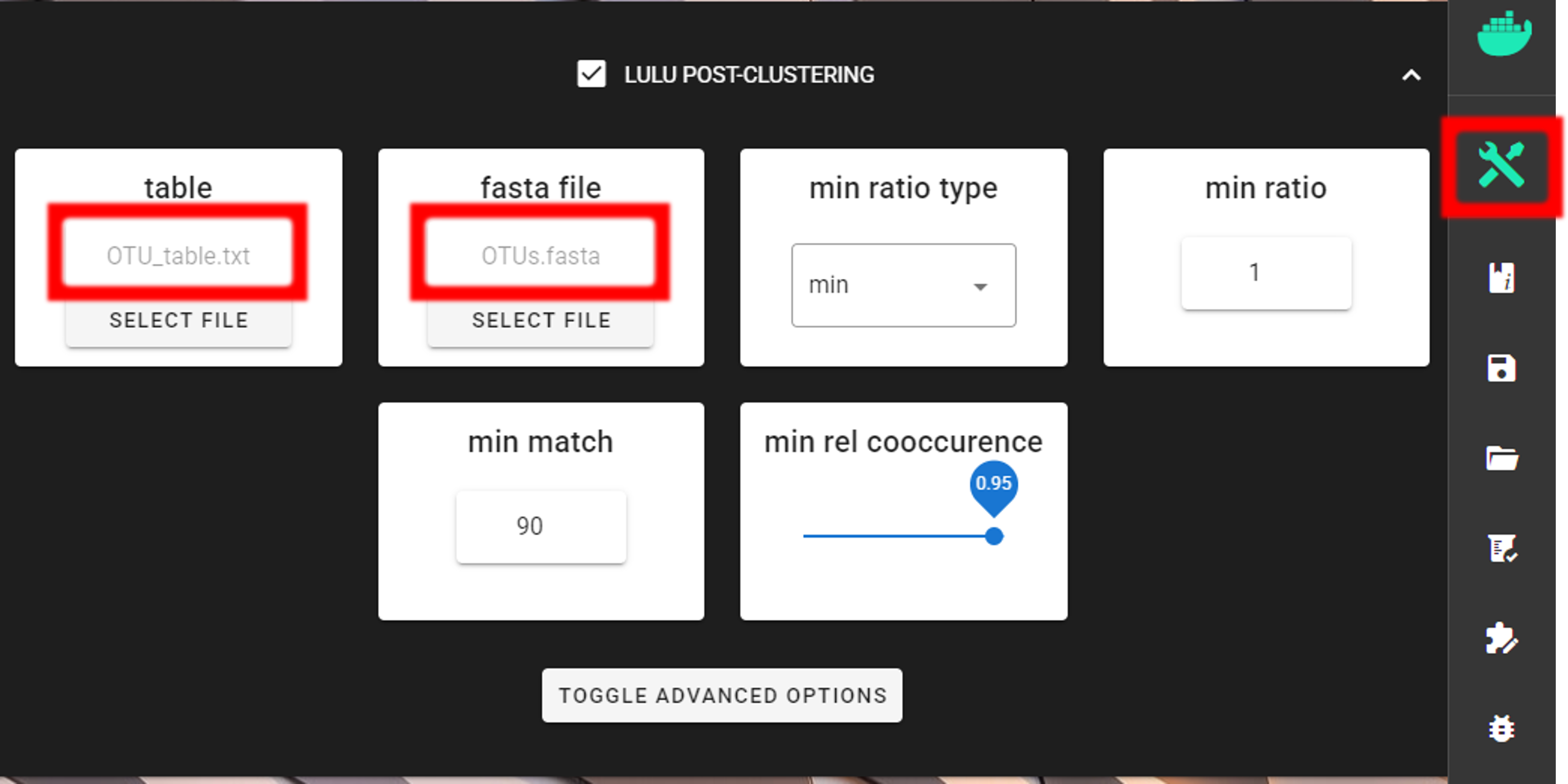
LULU post-clustering

Additionally, we can perform LULU post-clustering to merge co-occurring ‘daughter’ OTUs.

LULU description from the LULU repository: the purpose of LULU is to reduce the number of erroneous OTUs in OTU tables to achieve more realistic biodiversity metrics. By evaluating the co-occurence patterns of OTUs among samples LULU identifies OTUs that consistently satisfy some user selected criteria for being errors of more abundant OTUs and merges these. It has been shown that curation with LULU consistently result in more realistic diversity metrics.

Here, we are performing LULU post-clustering via QuickTools panel (on the right ribbon).

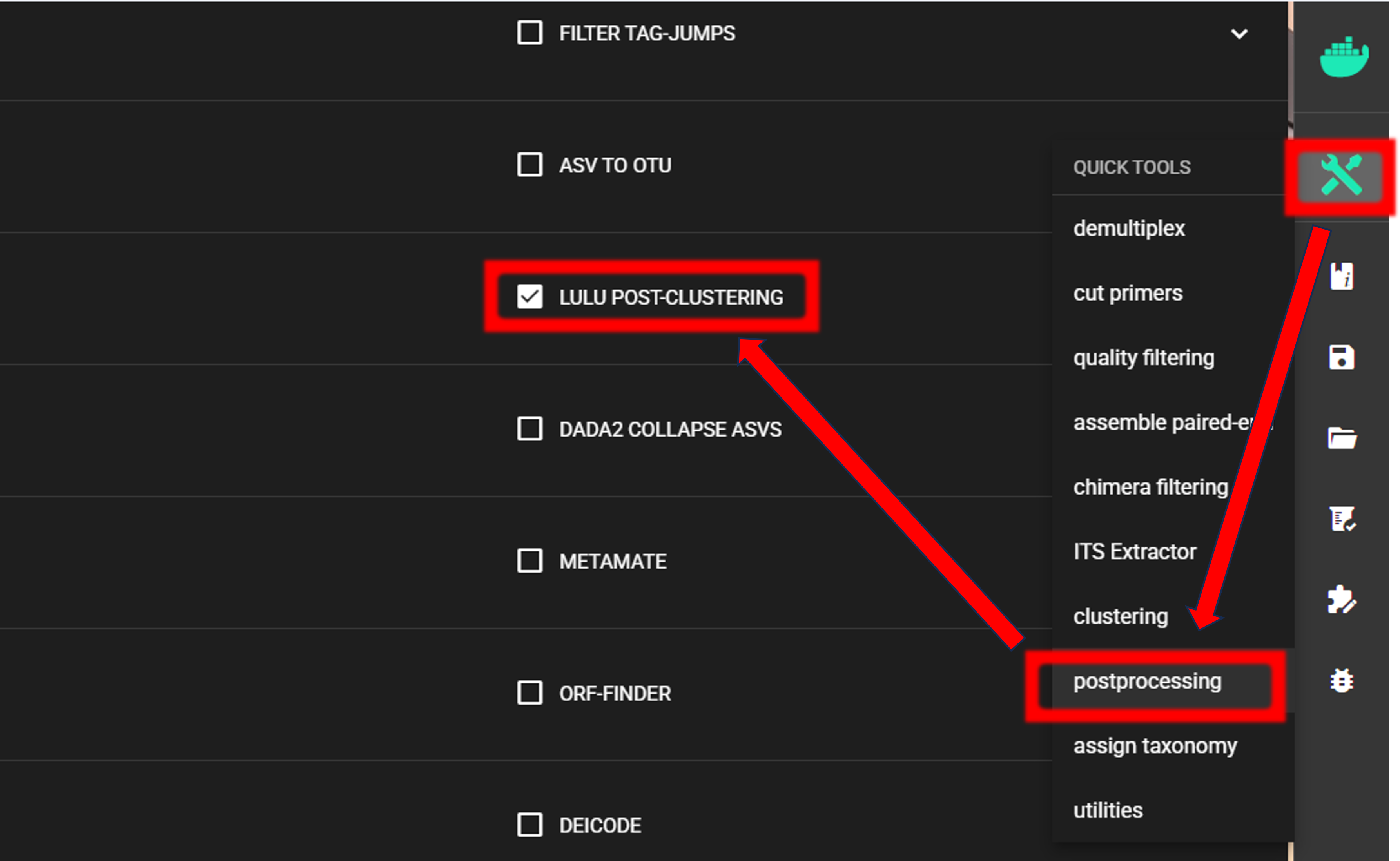
The input data are OTU_table_TagJumpFilt.txt and OTUs.fasta files in the clustering_out/curated directory.

Here, we are using the default settings (which are suitable for most cases), but feel free to experiment with various settings to see the effect on the results.

To START

To START, specify working directory under SELECT WORKDIR (outputs will be written here), but the following requests about Sequence files extension and Sequencing read types do not matter here, just click ‘Confirm’.

If postclustering merges some OTUs, then the outputs are:

Outputs in lulu_out directory:
OTU_table.lulu.txt	curated table in tab delimited txt format
OTUs.lulu.fasta	fasta file for the molecular units (OTUs or ASVs) in the curated table
match_list.lulu	match list file that was used by LULU to merge ‘daughter’ molecular units
discarded_units.lulu	molecular units (OTUs or ASVs) that were merged with other units based on specified thresholds

Did ‘postclustering with LULU’ have any effect?

In this example, we applied the postclustering step. The results of this is in the $WD/lulu_out folder (where $WD is the working directory). If we examine the README.txt file in that folder, then we see that “Total of 0 Features (OTUs/ASVs) were merged”, and therefore we do not have any OTU table or fasta file on the $WD/lulu_out folder.

Note that this is a small example dataset, but with larger datasets postclustering merges many ‘daughter’ OTUs into ‘parent’ OTUs.

---

Final OTU files

Now, final files are:

• clustering_out/curated/OTUs.fasta

• clustering_out/curated/OTU_table_TagJumpFilt_lenFilt.txt

• taxonomy_out.blast/BLAST_1st_hit_parsed.txt

Proceed with any relevant statistical analyses using the curated files.